
ABE, RSABE, ABEL
A Comparison
Helmut Schütz
April 5, 2024
Consider allowing JavaScript. Otherwise, you have to be proficient in
reading  since formulas
will not be rendered. Furthermore, the table of contents in the left
column for navigation will not be available and code-folding not
supported. Sorry for the inconvenience.
since formulas
will not be rendered. Furthermore, the table of contents in the left
column for navigation will not be available and code-folding not
supported. Sorry for the inconvenience.
Examples in this article were generated with
 4.3.3 by the packages
 PowerTOST version 1.5.6. 2024-03-18
1 and
TeachingDemos.2
More examples are given in the respective vignettes.3 4 See also the README on GitHub for an overview and the online manual5 for details.
For background about sample size estimations in replicate designs see the respective articles (ABE, RSABE, and ABEL). See also the articles about power and sensitivity analyses.
- The right-hand badges give the respective section’s ‘level’.
- Basics about power and sample size methodology – requiring no or only limited statistical expertise.
- These sections are the most important ones. They are – hopefully – easily comprehensible even for novices.
- A somewhat higher knowledge of statistics and/or R is required. May be skipped or reserved for a later reading.
- An advanced knowledge of statistics and/or R is required. Not recommended for beginners in particular.
- Click to show / hide R code.
- To copy R code to the clipboard click on
the icon
 in the top left corner.
| Abbreviation | Meaning |
|---|---|
| \(\small{\alpha}\) | Nominal level of the test, probability of Type I Error (patient’s risk) |
| (A)BE | (Average) Bioequivalence |
| ABEL | Average Bioequivalence with Expanding Limits |
| AUC | Area Under the Curve |
| \(\small{\beta}\) | Probability of Type II Error (producer’s risk), where \(\small{\beta=1-\pi}\) |
| CDE | Center for Drug Evaluation (China) |
| CI | Confidence Interval |
| CL | Confidence Limit |
| Cmax | Maximum concentration |
| \(\small{CV_\text{w}}\) | (Pooled) within-subject Coefficient of Variation |
| \(\small{CV_\text{wR},\;CV_\text{wT}}\) | Observed within-subject Coefficient of Variation of the Reference and Test product |
| \(\small{\Delta}\) | Clinically relevant difference |
| EMA | European Medicines Agency |
| FDA | (U.S.) Food and Drug Administration |
| \(\small{H_0}\) | Null hypothesis (inequivalence) |
| \(\small{H_1}\) | Alternative hypothesis (equivalence) |
| HVD(P) | Highly Variable Drug (Product) |
| \(\small{k}\) | Regulatory constant in ABEL (0.760) |
| \(\small{\mu_\text{T}/\mu_\text{R}}\) | True T/R-ratio |
| \(\small{n}\) | Sample size |
| \(\small{\pi}\) | (Prospective) power, where \(\small{\pi=1-\beta}\) |
| PE | Point Estimate |
| R | Reference product |
| RSABE | Reference-Scaled Average Bioequivalence |
| SABE | Scaled Average Bioequivalence |
| \(\small{s_\text{bR}^2,\;s_\text{bT}^2}\) | Observed between-subject variance of the Reference and Test product |
| \(\small{s_\text{wR},\;s_\text{wT}}\) | Observed within-subject standard deviation of the Reference and Test product |
| \(\small{s_\text{wR}^2,\;s_\text{wT}^2}\) | Observed within-subject variance of the Reference and Test product |
| \(\small{\sigma_\text{wR}}\) | True within-subject standard deviation of the Reference product |
| T | Test product |
| \(\small{\theta_0}\) | True T/R-ratio |
| \(\small{\theta_1,\;\theta_2}\) | Fixed lower and upper limits of the acceptance range (generally 80.00 – 125.00%) |
| \(\small{\theta_\text{s}}\) | Regulatory constant in RSABE (0.8925742…) |
| \(\small{\theta_{\text{s}_1},\;\theta_{\text{s}_2}}\) | Scaled lower and upper limits of the acceptance range |
| TIE | Type I Error (patient’s risk) |
| TIIE | Type II Error (producer’s risk: 1 – power) |
| uc | Upper cap of expansion in ABEL |
| 2×2×2 | 2-treatment 2-sequence 2-period crossover design (TR|RT) |
| 2×2×3 | 2-treatment 2-sequence 3-period full replicate designs (TRT|RTR and TTR|RRT) |
| 2×2×4 | 2-treatment 2-sequence 4-period full replicate designs (TRTR|RTRT, TRRT|RTTR, and TTRR|RRTT) |
| 2×3×3 | 2-treatment 3-sequence 3-period partial replicate design (TRR|RTR|RRT) |
| 2×4×2 | 2-treatment 4-sequence 2-period full replicate design (TR|RT|TT|RR) |
| 2×4×4 | 2-treatment 4-sequence 4-period full replicate designs (TRTR|RTRT|TRRT|RTTR and TRRT|RTTR|TTRR|RRTT) |
Introduction
What are the differences between Average Bioequivalence (ABE), Reference-Scaled Average Bioequivalence (RSABE), and Average Bioequivalence with Expanding Limits (ABEL) in terms of power and sample sizes?
For details about inferential statistics and hypotheses in equivalence see another article.
Terminology:
- A Highy Variable Drug (HVD) shows a within-subject Coefficient of Variation of the Reference (\(\small{CV_\text{wR}}\)) > 30% if administered as a solution in a replicate design. The high variability is an intrinsic property of the drug (absorption, permeation, clearance – in any combination).
- A Highy Variable Drug Product (HVDP) shows a \(\small{CV_\text{wR}}\) > 30% in a replicate design.6
The concept of Scaled Average Bioequivalence (SABE) for HVD(P)s is based on the following considerations:
- HVD(P)s are safe and efficacious despite their high
variability because:
- They have a wide therapeutic
index (i.e., a flat dose-response curve). Consequently,
even substantial changes in concentrations have only a limited impact on
the effect.
If they would have a narrow therapeutic index, adverse effects (due to high concentrations) and lacking effects (due to low concentrations) would have been observed in Phase II (or in Phase III at the latest) and therefore, the originator’s product would not have been approved in the first place.7 - Once approved, the product has a documented safety / efficacy record in phase IV and in clinical practice. If problems would became evident, the product would have been taken off the market.
- They have a wide therapeutic
index (i.e., a flat dose-response curve). Consequently,
even substantial changes in concentrations have only a limited impact on
the effect.
- Given that, the conventional ‘clinically relevant difference’ Δ of 20% in ABE (leading to the fixed limits of 80.00 – 125.00%) is considered overly conservative and therefore, requires large sample sizes.
- Thus, a more relaxed Δ > 20% was proposed. A natural approach is to scale (expand / widen) the limits based on the within-subject variability of the reference product σwR.8
The conventional confidence interval inclusion approach in ABE is based on \[\begin{matrix}\tag{1} \theta_1=1-\Delta,\theta_2=\left(1-\Delta\right)^{-1}\\ H_0:\;\frac{\mu_\text{T}}{\mu_\text{R}}\not\subset\left\{\theta_1,\,\theta_2\right\}\;vs\;H_1:\;\theta_1<\frac{\mu_\text{T}}{\mu_\text{R}}<\theta_2, \end{matrix}\] where \(\small{\Delta}\) is the clinically relevant difference, \(\small{\theta_1}\) and \(\small{\theta_2}\) are the fixed lower and upper limits of the acceptance range, \(\small{H_0}\) is the null hypothesis of inequivalence, and \(\small{H_1}\) is the alternative hypothesis of equivalence. \(\small{\mu_\text{T}}\) and \(\small{\mu_\text{R}}\) are the geometric least squares means of \(\small{\text{T}}\) and \(\small{\text{R}}\), respectively.
\(\small{(1)}\) is modified in Scaled Average Bioequivalence (SABE) to \[H_0:\;\frac{\mu_\text{T}}{\mu_\text{R}}\Big{/}\sigma_\text{wR}\not\subset\left\{\theta_{\text{s}_1},\,\theta_{\text{s}_2}\right\}\;vs\;H_1:\;\theta_{\text{s}_1}<\frac{\mu_\text{T}}{\mu_\text{R}}\Big{/}\sigma_\text{wR}<\theta_{\text{s}_2},\tag{2}\] where \(\small{\sigma_\text{wR}}\) is the standard deviation of the reference. The scaled limits \(\small{\left\{\theta_{\text{s}_1},\,\theta_{\text{s}_2}\right\}}\) of the acceptance range depend on conditions given by the agency.
RSABE is recommended by the FDA and China’s CDE. ABEL is another variant of SABE and recommended in all other jurisdictions.
In order to apply the methods9 following conditions have to be fulfilled:
- The study has to be performed in a replicate design, i.e.,
at least the reference product has to be administered twice.
Realization: Observations (in a sample) of a random variable (of the population).
- The realized within-subject variability of the reference
has to be high
(in RSABE swR ≥ 0.29410 and in ABEL CVwR > 30%). - ABEL
only:
- A clinical justification must be given that the expanded limits will not impact safety / efficacy.
- There is an ‘upper cap’ of scaling (uc = 50%, except for Health Canada, where uc ≈ 57.382%11), i.e., the expansion is limited to 69.84 – 143.19% or 67.7 – 150.0%, respectively.
- Except for applications in Brazil and Chile, it has to be demonstrated that the high variability of the reference is not caused by ‘outliers’.
In all methods a point estimate-constraint is imposed. Even if a study would pass the scaled limits, the PE has to lie within 80.00 – 125.00% in order to pass.
It should be noted that larger deviations between geometric mean
ratios arise as a natural, direct consequence of the higher
variability.
Since extreme values are common for
HVD(P)s,
assessment of ‘outliers’ is not required by the
FDA and China’s
CDE for
RSABE, as
well as by Brazil’s
ANVISA and
Chile’s ANAMED for
ABEL.
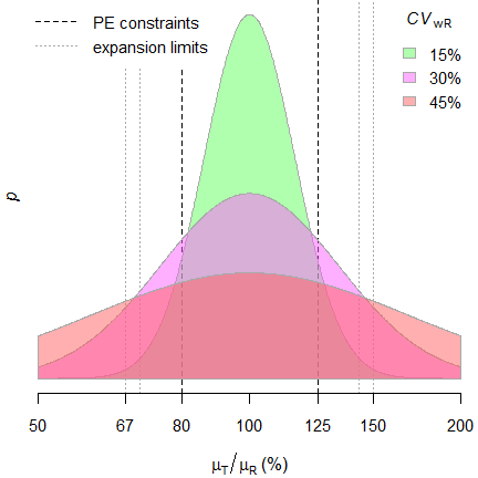
Fig. 1 Distribution of geometric
mean ratios.
The PE-constraint – together with the upper cap of expansion in jurisdictions applying ABEL – lead to truncated distributions. Hence, the test assuming the normal distribution of \(\small{\log_{e}}\)-transformed data is not correct in the strict sense.
Preliminaries
A basic knowledge of R is
required. To run the scripts at least version 1.4.8 (2019-08-29) of
PowerTOST is required and at least 1.5.3 (2021-01-18)
suggested. Any version of R would likely do,
though the current release of PowerTOST was only tested
with version 4.2.3 (2023-03-15) and later.
All scripts were run on a Xeon E3-1245v3 @ 3.40GHz (1/4 cores) 16GB RAM
with R 4.3.3 on Windows 7 build 7601, Service
Pack 1, Universal C Runtime 10.0.10240.16390.
library(PowerTOST)     # attach the packages
library(TeachingDemos) # to run the examplesSample size
The idea behind reference-scaling is to the avoid extreme sample sizes required for ABE and preserve power independent from the \(\small{CV}\).
Let’s explore some examples. I assumed a \(\small{CV}\) of 0.45, a T/R-ratio (\(\small{\theta_0}\)) of 0.90, and targeted
≥ 80% power in some common replicate designs.
Note that sample sizes are integers and follow a
staircase
function because in software packages balanced sequences are
returned.
CV      <- 0.45
theta0  <- 0.90
target  <- 0.80
designs <- c("2x2x4", "2x2x3", "2x3x3")
method  <- c("ABE", "ABEL", "RSABE")
res     <- data.frame(design = rep(designs, each = length(method)),
                      method = method, n = NA)
for (i in 1:nrow(res)) {
  if (res$method[i] == "ABE") {
    res[i, 3] <- sampleN.TOST(CV = CV, theta0 = theta0,
                              design = res$design[i],
                              targetpower = target,
                              print = FALSE)[["Sample size"]]
  }
  if (res$method[i] == "ABEL") {
    res[i, 3] <- sampleN.scABEL(CV = CV, theta0 = theta0,
                                design = res$design[i],
                                targetpower = target,
                                print = FALSE,
                                details = FALSE)[["Sample size"]]
  }
  if (res$method[i] == "RSABE") {
    res[i, 3] <- sampleN.RSABE(CV = CV, theta0 = theta0,
                               design = res$design[i],
                               targetpower = target,
                               print = FALSE,
                               details = FALSE)[["Sample size"]]
  }
}
print(res, row.names = FALSE)
#  design method   n
#   2x2x4    ABE  84
#   2x2x4   ABEL  28
#   2x2x4  RSABE  24
#   2x2x3    ABE 124
#   2x2x3   ABEL  42
#   2x2x3  RSABE  36
#   2x3x3    ABE 126
#   2x3x3   ABEL  39
#   2x3x3  RSABE  33
CV <- 0.45
theta0 <- seq(0.95, 0.85, -0.001)
methods <- c("ABE", "ABEL", "RSABE")
clr <- c("red", "magenta", "blue")
ylab <- paste0("sample size (CV = ", 100*CV, "%)")
#################
design <- "2x2x4"
res1 <- data.frame(theta0 = theta0,
method = rep(methods, each =length(theta0)),
n = NA)
for (i in 1:nrow(res1)) {
if (res1$method[i] == "ABE") {
res1$n[i] <- sampleN.TOST(CV = CV, theta0 = res1$theta0[i],
design = design,
print = FALSE)[["Sample size"]]
}
if (res1$method[i] == "ABEL") {
res1$n[i] <- sampleN.scABEL(CV = CV, theta0 = res1$theta0[i],
design = design, print = FALSE,
details = FALSE)[["Sample size"]]
}
if (res1$method[i] == "RSABE") {
res1$n[i] <- sampleN.RSABE(CV = CV, theta0 = res1$theta0[i],
design = design, print = FALSE,
details = FALSE)[["Sample size"]]
}
}
dev.new(width = 4.5, height = 4.5, record = TRUE)
op <- par(no.readonly = TRUE)
par(lend = 2, ljoin = 1, mar = c(4, 3.3, 0.1, 0.2), cex.axis = 0.9)
plot(theta0, res1$n[res1$method == "ABE"], type = "n", axes = FALSE,
ylim = c(12, max(res1$n)), xlab = expression(theta[0]),
log = "xy", ylab = "")
abline(v = seq(0.85, 0.95, 0.025), lty = 3, col = "lightgrey")
abline(v = 0.90, lty = 2)
abline(h = axTicks(2, log = TRUE), lty = 3, col = "lightgrey")
axis(1, at = seq(0.85, 0.95, 0.025))
axis(2, las = 1)
mtext(ylab, 2, line = 2.4)
legend("bottomleft", legend = methods, inset = 0.02, lwd = 2, cex = 0.9,
col = clr, box.lty = 0, bg = "white", title = "\u226580% power")
lines(theta0, res1$n[res1$method == "ABE"],
type = "S", lwd = 2, col = clr[1])
lines(theta0, res1$n[res1$method == "ABEL"],
type = "S", lwd = 2, col = clr[2])
lines(theta0, res1$n[res1$method == "RSABE"],
type = "S", lwd = 2, col = clr[3])
box()
#################
design <- "2x2x3"
res2 <- data.frame(theta0 = theta0,
method = rep(methods, each =length(theta0)),
n = NA)
for (i in 1:nrow(res2)) {
if (res2$method[i] == "ABE") {
res2$n[i] <- sampleN.TOST(CV = CV, theta0 = res2$theta0[i],
design = design,
print = FALSE)[["Sample size"]]
}
if (res2$method[i] == "ABEL") {
res2$n[i] <- sampleN.scABEL(CV = CV, theta0 = res2$theta0[i],
design = design, print = FALSE,
details = FALSE)[["Sample size"]]
}
if (res2$method[i] == "RSABE") {
res2$n[i] <- sampleN.RSABE(CV = CV, theta0 = res2$theta0[i],
design = design, print = FALSE,
details = FALSE)[["Sample size"]]
}
}
plot(theta0, res2$n[res2$method == "ABE"], type = "n", axes = FALSE,
ylim = c(12, max(res2$n)), xlab = expression(theta[0]),
log = "xy", ylab = "")
abline(v = seq(0.85, 0.95, 0.025), lty = 3, col = "lightgrey")
abline(v = 0.90, lty = 2)
abline(h = axTicks(2, log = TRUE), lty = 3, col = "lightgrey")
axis(1, at = seq(0.85, 0.95, 0.025))
axis(2, las = 1)
mtext(ylab, 2, line = 2.4)
legend("bottomleft", legend = methods, inset = 0.02, lwd = 2, cex = 0.9,
col = clr, box.lty = 0, bg = "white", title = "\u226580% power")
lines(theta0, res2$n[res2$method == "ABE"],
type = "S", lwd = 2, col = clr[1])
lines(theta0, res2$n[res2$method == "ABEL"],
type = "S", lwd = 2, col = clr[2])
lines(theta0, res2$n[res2$method == "RSABE"],
type = "S", lwd = 2, col = clr[3])
box()
#################
design <- "2x3x3"
res3 <- data.frame(theta0 = theta0,
method = rep(methods, each =length(theta0)),
n = NA)
for (i in 1:nrow(res3)) {
if (res3$method[i] == "ABE") {
res3$n[i] <- sampleN.TOST(CV = CV, theta0 = res3$theta0[i],
design = design,
print = FALSE)[["Sample size"]]
}
if (res3$method[i] == "ABEL") {
res3$n[i] <- sampleN.scABEL(CV = CV, theta0 = res3$theta0[i],
design = design, print = FALSE,
details = FALSE)[["Sample size"]]
}
if (res3$method[i] == "RSABE") {
res3$n[i] <- sampleN.RSABE(CV = CV, theta0 = res3$theta0[i],
design = design, print = FALSE,
details = FALSE)[["Sample size"]]
}
}
plot(theta0, res3$n[res3$method == "ABE"], type = "n", axes = FALSE,
ylim = c(12, max(res3$n)), xlab = expression(theta[0]),
log = "xy", ylab = "")
abline(v = seq(0.85, 0.95, 0.025), lty = 3, col = "lightgrey")
abline(v = 0.90, lty = 2)
abline(h = axTicks(2, log = TRUE), lty = 3, col = "lightgrey")
axis(1, at = seq(0.85, 0.95, 0.025))
axis(2, las = 1)
mtext(ylab, 2, line = 2.4)
legend("bottomleft", legend = methods, inset = 0.02, lwd = 2, cex = 0.9,
col = clr, box.lty = 0, bg = "white", title = "\u226580% power")
lines(theta0, res3$n[res3$method == "ABE"],
type = "S", lwd = 2, col = clr[1])
lines(theta0, res3$n[res3$method == "ABEL"],
type = "S", lwd = 2, col = clr[2])
lines(theta0, res3$n[res3$method == "RSABE"],
type = "S", lwd = 2, col = clr[3])
box()
par(op)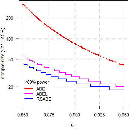
Fig. 2 4-period full replicate design.
It’s obvious that we need substantially smaller sample sizes in the methods for reference-scaling than we would require for ABE. The sample size functions of the scaling methods are also not that steep, which means that even if our assumptions about the T/R-ratio would be wrong, power (and hence, sample sizes) would be affected to a lesser degree.
Nevertheless, one should not be overly optimistic about the
T/R-ratio. For
HVD(P)s a
T/R-ratio of ‘better’ than 0.90 should be avoided.12
NB, that’s the reason why in
sampleN.scABEL() and sampleN.RSABE() the
default is theta0 = 0.90. If scaling is not acceptable
(i.e., AUC for the
EMA and
Cmax for Health Canada), I strongly recommend to
specify theta0 = 0.90 in sampleN.TOST()
because its default is 0.95.
Note that RSABE is more permissive than ABEL due to its regulatory constant ≈0.8926 instead of 0.760 and unlimited scaling (no upper cap). Hence, sample sizes for RSABE are always smaller than the ones for ABEL.
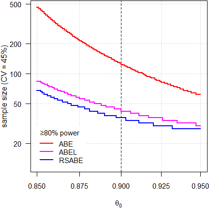
Fig. 3 3-period full replicate design.
Since power depends on the number of treatments, roughly 50% more subjects are required than in 4-period full replicate designs.
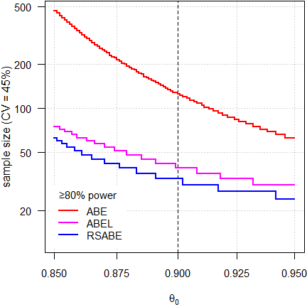
Fig. 4 Partial replicate design.
Similar sample sizes than in the 3-period full replicate design because both have the same degrees of freedom. However, the step size is wider (three sequences instead of two).
Before we estimate a sample size, we have to be clear about the planned evaluation. The EMA and most other agencies require an ANOVA (i.e., all effects fixed), whereas Health Canada, the FDA, and China’s CDE a mixed-effects model.
Let’s explore the replicate designs implemented in
PowerTOST. Note that only
ABE for Balaam’s design
(TR|RT|TT|RR) is implemented.
print(known.designs()[7:11, c(2:4, 9)], row.names = FALSE) # relevant columns# design df df2 name
# 2x2x3 2*n-3 n-2 2x2x3 replicate crossover
# 2x2x4 3*n-4 n-2 2x2x4 replicate crossover
# 2x4x4 3*n-4 n-4 2x4x4 replicate crossover
# 2x3x3 2*n-3 n-3 partial replicate (2x3x3)
# 2x4x2 n-2 n-2 Balaam's (2x4x2)The column df gives the degrees of freedom of an
ANOVA and the column
df2 the ones of a mixed-effects model.
Which model is intended for evaluation is controlled by the argument
robust, which is FALSE (for an
ANOVA) by default. If set to
TRUE, the estimation will be performed for a mixed-effects
model.
A simple example (T/R-ratio 0.90, CV 0.25 – 0.50, 2×2×4 design targeted at power 0.80:
theta0          <- 0.90
CV              <- seq(0.25, 0.5, 0.05)
design          <- "2x2x4"
target          <- 0.80
reg1            <- reg_const(regulator = "EMA")
reg1$name       <- "USER"
reg1$est_method <- "ISC" # keep conditions but change from "ANOVA"
reg2            <- reg_const("USER", r_const = log(1.25) / 0.25,
                             CVswitch = 0.3, CVcap = Inf) # ANOVA
#####################################################
# Note: These are internal (not exported) functions #
# Use them only if you know what you are doing!     #
#####################################################
d.no   <- PowerTOST:::.design.no(design)
ades   <- PowerTOST:::.design.props(d.no)
df1    <- PowerTOST:::.design.df(ades, robust = FALSE)
df2    <- PowerTOST:::.design.df(ades, robust = TRUE)
ns     <- nu <- data.frame(CV = CV, ABE.fix = NA_integer_,
                           ABE.mix = NA_integer_, ABEL.fix = NA_integer_,
                           ABEL.mix = NA_integer_, RSABE.fix = NA_integer_,
                           RSABE.mix = NA_integer_)
for (i in seq_along(CV)) {
  ns$ABE.fix[i]   <- sampleN.TOST(CV = CV[i], theta0 = theta0,
                                  targetpower = target, design = design,
                                  print = FALSE,
                                  details = FALSE)[["Sample size"]]
  n               <- ns$ABE.fix[i]
  nu$ABE.fix[i]   <- eval(df1)
  ns$ABE.mix[i]   <- sampleN.TOST(CV = CV[i], theta0 = theta0,
                                  targetpower = target, design = design,
                                  robust = TRUE,
                                  print = FALSE,
                                  details = FALSE)[["Sample size"]]
  n               <- ns$ABE.mix[i]
  nu$ABE.mix[i]   <- eval(df2)
  ns$ABEL.fix[i]  <- sampleN.scABEL(CV = CV[i], theta0 = theta0,
                                    targetpower = target, design = design,
                                    print = FALSE,
                                    details = FALSE)[["Sample size"]]
  n               <- ns$ABEL.fix[i]
  nu$ABEL.fix[i]  <- eval(df1)
  ns$ABEL.mix[i]  <- sampleN.scABEL(CV = CV[i], theta0 = theta0,
                                    targetpower = target, design = design,
                                    regulator = reg1,
                                    print = FALSE,
                                    details = FALSE)[["Sample size"]]
  n               <- ns$ABEL.mix[i]
  nu$ABEL.mix[i]  <- eval(df2)
  ns$RSABE.fix[i] <- sampleN.scABEL(CV = CV[i], theta0 = theta0,
                                    targetpower = target, design = design,
                                    regulator = reg2,
                                    print = FALSE,
                                    details = FALSE)[["Sample size"]]
  n               <- ns$RSABE.fix[i]
  nu$RSABE.fix[i] <- eval(df1)
  ns$RSABE.mix[i] <- sampleN.RSABE(CV = CV[i], theta0 = theta0,
                                   targetpower = target, design = design,
                                   print = FALSE,
                                   details = FALSE)[["Sample size"]]
  n               <- ns$RSABE.mix[i]
  nu$RSABE.mix[i] <- eval(df2)
}
cat("Sample sizes\n")
print(ns, row.names = FALSE)
# Sample sizes
# CV ABE.fix ABE.mix ABEL.fix ABEL.mix RSABE.fix RSABE.mix
# 0.25 28 30 28 30 28 28
# 0.30 40 40 34 36 28 32
# 0.35 52 54 34 36 24 28
# 0.40 68 68 30 32 22 24
# 0.45 84 84 28 30 20 24
# 0.50 100 102 28 30 20 22For the mixed-effects models sample sizes are in general slightly larger.
cat("Degrees of freedom\n")
print(nu, row.names = FALSE)
# Degrees of freedom
# CV ABE.fix ABE.mix ABEL.fix ABEL.mix RSABE.fix RSABE.mix
# 0.25 80 28 80 28 80 26
# 0.30 116 38 98 34 80 30
# 0.35 152 52 98 34 68 26
# 0.40 200 66 86 30 62 22
# 0.45 248 82 80 28 56 22
# 0.50 296 100 80 28 56 20In the mixed-effects models we have fewer degrees of freedom (more
effects are estimated).
Note that for the
FDA’s
RSABE
always a mixed-effects model has to be employed and thus, the results
for an ANOVA are given only
for comparison.
Power
Let’s change the point of view. As above, I assumed \(\small{CV=0.45}\), \(\small{\theta_0=0.90}\), and targeted ≥ 80% power. This time I explored how \(\small{CV}\) different from my assumption affects power with the estimated sample size.
Additionally I assessed ‘pure’ SABE, i.e., without an upper cap of scaling and without the PE-constraint for the EMA’s conditions (switching \(\small{CV_\text{wR}=30\%}\), regulatory constant \(\small{k=0.760}\)).
CV      <- 0.45
theta0  <- 0.90
target  <- 0.80
designs <- c("2x2x4", "2x2x3", "2x3x3")
method  <- c("ABE", "ABEL", "RSABE", "SABE")
# Pure SABE (only for comparison)
# No upper cap of scaling, no PE constraint
pure    <- reg_const("USER",
                     r_const  = 0.760,
                     CVswitch = 0.30,
                     CVcap    = Inf)
pure$pe_constr <- FALSE
res     <- data.frame(design = rep(designs, each = length(method)),
                      method = method, n = NA, power = NA,
                      CV0.40 = NA, CV0.50 = NA)
for (i in 1:nrow(res)) {
  if (res$method[i] == "ABE") {
    res[i, 3:4] <- sampleN.TOST(CV = CV, theta0 = theta0,
                                design = res$design[i],
                                targetpower = target,
                                print = FALSE)[7:8]
    res[i, 5]   <- power.TOST(CV = 0.4, theta0 = theta0,
                              n = res[i, 3],
                              design = res$design[i])
    res[i, 6]   <- power.TOST(CV = 0.5, theta0 = theta0,
                              n = res[i, 3],
                              design = res$design[i])
  }
  if (res$method[i] == "ABEL") {
    res[i, 3:4] <- sampleN.scABEL(CV = CV, theta0 = theta0,
                                  design = res$design[i],
                                  targetpower = target,
                                  print = FALSE,
                                  details = FALSE)[8:9]
    res[i, 5]   <- power.scABEL(CV = 0.4, theta0 = theta0,
                                n = res[i, 3],
                                design = res$design[i])
    res[i, 6]   <- power.scABEL(CV = 0.5, theta0 = theta0,
                                n = res[i, 3],
                                design = res$design[i])
  }
  if (res$method[i] == "RSABE") {
    res[i, 3:4] <- sampleN.RSABE(CV = CV, theta0 = theta0,
                                 design = res$design[i],
                                 targetpower = target,
                                 print = FALSE,
                                 details = FALSE)[8:9]
    res[i, 5]   <- power.RSABE(CV = 0.4, theta0 = theta0,
                               n = res[i, 3],
                               design = res$design[i])
    res[i, 6]   <- power.RSABE(CV = 0.5, theta0 = theta0,
                               n = res[i, 3],
                               design = res$design[i])
  }
  if (res$method[i] == "SABE") {
    res[i, 3:4] <- sampleN.scABEL(CV = CV, theta0 = theta0,
                                  design = res$design[i],
                                  targetpower = target,
                                  regulator = pure,
                                  print = FALSE,
                                  details = FALSE)[8:9]
    res[i, 5]   <- power.scABEL(CV = 0.4, theta0 = theta0,
                                n = res[i, 3],
                                design = res$design[i],
                                regulator = pure)
    res[i, 6]   <- power.scABEL(CV = 0.5, theta0 = theta0,
                                n = res[i, 3],
                                design = res$design[i],
                                regulator = pure)
  }
}
res[, 4:6] <- signif(res[, 4:6], 5)
print(res, row.names = FALSE)
# design method n power CV0.40 CV0.50
# 2x2x4 ABE 84 0.80569 0.87483 0.73700
# 2x2x4 ABEL 28 0.81116 0.78286 0.81428
# 2x2x4 RSABE 24 0.82450 0.80516 0.83001
# 2x2x4 SABE 28 0.81884 0.78415 0.84388
# 2x2x3 ABE 124 0.80012 0.87017 0.73102
# 2x2x3 ABEL 42 0.80017 0.77676 0.80347
# 2x2x3 RSABE 36 0.81147 0.79195 0.81888
# 2x2x3 SABE 42 0.80961 0.77868 0.83463
# 2x3x3 ABE 126 0.80570 0.87484 0.73701
# 2x3x3 ABEL 39 0.80588 0.77587 0.80763
# 2x3x3 RSABE 33 0.82802 0.80845 0.83171
# 2x3x3 SABE 39 0.81386 0.77650 0.84100# Cave: very long runtime
CV.fix <- 0.45
CV <- seq(0.35, 0.55, length.out = 201)
theta0 <- 0.90
methods <- c("ABE", "ABEL", "RSABE", "SABE")
clr <- c("red", "magenta", "blue", "#00800080")
# Pure SABE (only for comparison)
# No upper cup of scaling, no PE constraint
pure <- reg_const("USER",
r_const = 0.760,
CVswitch = 0.30,
CVcap = Inf)
pure$pe_constr <- FALSE
#################
design <- "2x2x4"
res1 <- data.frame(CV = CV,
method = rep(methods, each =length(CV)),
power = NA)
n.ABE <- sampleN.TOST(CV = CV.fix, theta0 = theta0,
design = design,
print = FALSE)[["Sample size"]]
n.RSABE <- sampleN.RSABE(CV = CV.fix, theta0 = theta0,
design = design, print = FALSE,
details = FALSE)[["Sample size"]]
n.ABEL <- sampleN.scABEL(CV = CV.fix, theta0 = theta0,
design = design, print = FALSE,
details = FALSE)[["Sample size"]]
n.SABE <- sampleN.scABEL(CV = CV.fix, theta0 = theta0,
design = design, print = FALSE,
regulator = pure,
details = FALSE)[["Sample size"]]
for (i in 1:nrow(res1)) {
if (res1$method[i] == "ABE") {
res1$power[i] <- power.TOST(CV = res1$CV[i], theta0 = theta0,
n = n.ABE, design = design)
}
if (res1$method[i] == "ABEL") {
res1$power[i] <- power.scABEL(CV = res1$CV[i], theta0 = theta0,
n = n.ABEL, design = design, nsims = 1e6)
}
if (res1$method[i] == "RSABE") {
res1$power[i] <- power.RSABE(CV = res1$CV[i], theta0 = theta0,
n = n.RSABE, design = design, nsims = 1e6)
}
if (res1$method[i] == "SABE") {
res1$power[i] <- power.scABEL(CV = res1$CV[i], theta0 = theta0,
n = n.ABEL, design = design,
regulator = pure, nsims = 1e6)
}
}
dev.new(width = 4.5, height = 4.5, record = TRUE)
op <- par(no.readonly = TRUE)
par(mar = c(4, 3.3, 0.1, 0.1), cex.axis = 0.9)
plot(CV, res1$power[res1$method == "ABE"], type = "n", axes = FALSE,
ylim = c(0.65, 1), xlab = "CV", ylab = "")
abline(v = seq(0.35, 0.55, 0.05), lty = 3, col = "lightgrey")
abline(v = 0.45, lty = 2)
abline(h = axTicks(2, log = FALSE), lty = 3, col = "lightgrey")
axis(1, at = seq(0.35, 0.55, 0.05))
axis(2, las = 1)
mtext("power", 2, line = 2.6)
legend("topright", legend = methods, inset = 0.02, lwd = 2, cex = 0.9,
col = clr, box.lty = 0, bg = "white", title = "n for CV = 45%")
lines(CV, res1$power[res1$method == "ABE"], lwd = 2, col = clr[1])
lines(CV, res1$power[res1$method == "ABEL"], lwd = 2, col = clr[2])
lines(CV, res1$power[res1$method == "RSABE"], lwd = 2, col = clr[3])
lines(CV, res1$power[res1$method == "SABE"], lwd = 2, col = clr[4])
box()
#################
design <- "2x2x3"
res2 <- data.frame(CV = CV,
method = rep(methods, each =length(CV)),
power = NA)
n.ABE <- sampleN.TOST(CV = CV.fix, theta0 = theta0,
design = design,
print = FALSE)[["Sample size"]]
n.RSABE <- sampleN.RSABE(CV = CV.fix, theta0 = theta0,
design = design, print = FALSE,
details = FALSE)[["Sample size"]]
n.ABEL <- sampleN.scABEL(CV = CV.fix, theta0 = theta0,
design = design, print = FALSE,
details = FALSE)[["Sample size"]]
n.SABE <- sampleN.scABEL(CV = CV.fix, theta0 = theta0,
design = design, print = FALSE,
regulator = pure,
details = FALSE)[["Sample size"]]
for (i in 1:nrow(res2)) {
if (res2$method[i] == "ABE") {
res2$power[i] <- power.TOST(CV = res2$CV[i], theta0 = theta0,
n = n.ABE, design = design)
}
if (res2$method[i] == "ABEL") {
res2$power[i] <- power.scABEL(CV = res2$CV[i], theta0 = theta0,
n = n.ABEL, design = design, nsims = 1e6)
}
if (res2$method[i] == "RSABE") {
res2$power[i] <- power.RSABE(CV = res2$CV[i], theta0 = theta0,
n = n.RSABE, design = design, nsims = 1e6)
}
if (res2$method[i] == "SABE") {
res2$power[i] <- power.scABEL(CV = res2$CV[i], theta0 = theta0,
n = n.ABEL, design = design,
regulator = pure, nsims = 1e6)
}
}
plot(CV, res2$power[res2$method == "ABE"], type = "n", axes = FALSE,
ylim = c(0.65, 1), xlab = "CV", ylab = "")
abline(v = seq(0.35, 0.55, 0.05), lty = 3, col = "lightgrey")
abline(v = 0.45, lty = 2)
abline(h = axTicks(2, log = FALSE), lty = 3, col = "lightgrey")
axis(1, at = seq(0.35, 0.55, 0.05))
axis(2, las = 1)
mtext("power", 2, line = 2.6)
legend("topright", legend = methods, inset = 0.02, lwd = 2, cex = 0.9,
col = clr, box.lty = 0, bg = "white", title = "n for CV = 45%")
lines(CV, res2$power[res2$method == "ABE"], lwd = 2, col = clr[1])
lines(CV, res2$power[res2$method == "ABEL"], lwd = 2, col = clr[2])
lines(CV, res2$power[res2$method == "RSABE"], lwd = 2, col = clr[3])
lines(CV, res2$power[res2$method == "SABE"], lwd = 2, col = clr[4])
box()
#################
design <- "2x3x3"
res3 <- data.frame(CV = CV,
method = rep(methods, each =length(CV)),
power = NA)
n.ABE <- sampleN.TOST(CV = CV.fix, theta0 = theta0,
design = design,
print = FALSE)[["Sample size"]]
n.RSABE <- sampleN.RSABE(CV = CV.fix, theta0 = theta0,
design = design, print = FALSE,
details = FALSE)[["Sample size"]]
n.ABEL <- sampleN.scABEL(CV = CV.fix, theta0 = theta0,
design = design, print = FALSE,
details = FALSE)[["Sample size"]]
n.SABE <- sampleN.scABEL(CV = CV.fix, theta0 = theta0,
design = design, print = FALSE,
regulator = pure,
details = FALSE)[["Sample size"]]
for (i in 1:nrow(res3)) {
if (res3$method[i] == "ABE") {
res3$power[i] <- power.TOST(CV = res3$CV[i], theta0 = theta0,
n = n.ABE, design = design)
}
if (res3$method[i] == "ABEL") {
res3$power[i] <- power.scABEL(CV = res3$CV[i], theta0 = theta0,
n = n.ABEL, design = design, nsims = 1e6)
}
if (res3$method[i] == "RSABE") {
res3$power[i] <- power.RSABE(CV = res3$CV[i], theta0 = theta0,
n = n.RSABE, design = design, nsims = 1e6)
}
if (res3$method[i] == "SABE") {
res3$power[i] <- power.scABEL(CV = res3$CV[i], theta0 = theta0,
n = n.ABEL, design = design,
regulator = pure, nsims = 1e6)
}
}
plot(CV, res3$power[res3$method == "ABE"], type = "n", axes = FALSE,
ylim = c(0.65, 1), xlab = "CV", ylab = "")
abline(v = seq(0.35, 0.55, 0.05), lty = 3, col = "lightgrey")
abline(v = 0.45, lty = 2)
abline(h = axTicks(2, log = FALSE), lty = 3, col = "lightgrey")
axis(1, at = seq(0.35, 0.55, 0.05))
axis(2, las = 1)
mtext("power", 2, line = 2.6)
legend("topright", legend = methods, inset = 0.02, lwd = 2, cex = 0.9,
col = clr, box.lty = 0, bg = "white", title = "n for CV = 45%")
lines(CV, res3$power[res3$method == "ABE"], lwd = 2, col = clr[1])
lines(CV, res3$power[res3$method == "ABEL"], lwd = 2, col = clr[2])
lines(CV, res3$power[res3$method == "RSABE"], lwd = 2, col = clr[3])
lines(CV, res3$power[res3$method == "SABE"], lwd = 2, col = clr[4])
box()
par(op)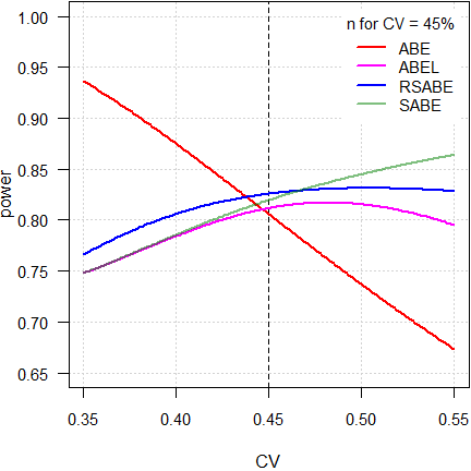
Fig. 5 4-period full replicate design.
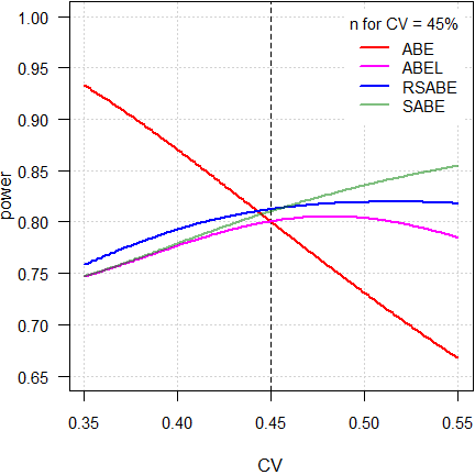
Fig. 6 3-period full replicate design.
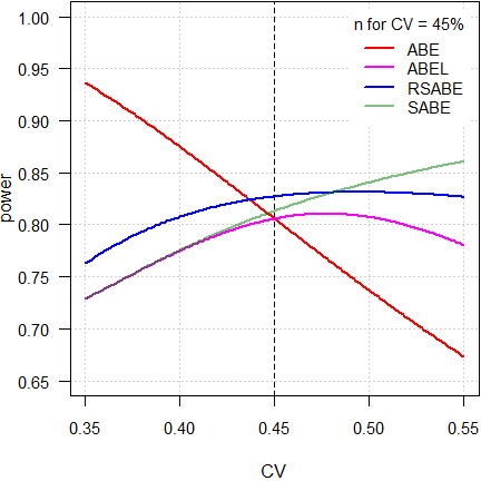
Fig. 7 Partial replicate design.
As expected, power of ABE is extremely dependent on the CV. Not surprising, because the acceptance limits are fixed at 80.00 – 125.00%.
As stated above, ideally reference-scaling should preserve power independent from the CV. If that would be the case, power would be a line parallel to the x-axis. However, the methods implemented by authorities are decision schemes (outlined in the articles about RSABE and ABEL), where certain conditions have to be observed. Therefore, beyond a maximum around 50%, power starts to decrease because the PE-constraint becomes increasingly important and – for ABEL – the upper cap of scaling sets in.
On the other hand, ‘pure’ SABE shows the unconstrained behavior of ABEL.
Let’s go deeper into the matter. As above but a wider range of CV values (0.3 – 1).
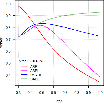
Fig. 8 4-period full replicate design.
Here we see a clear difference between
RSABE and
ABEL.
Although in both the PE-constraint
has to be observed, in the former no upper cap of scaling is imposed and
hence, power affected to a minor degree.
On the contrary, due to the upper upper cap of scaling in the latter, it
behaves similarly to ABE
with fixed limits of 69.84 – 143.19%.
Consequently, if the CV will be substantially larger than assumed, in ABEL power may be compromised.
Note also the huge gap between ABEL and ‘pure’ SABE. Whilst the PE-constraint is statistically not justified, it was introduced in all jurisdictions ‘for political reasons’.
“
- There is no scientific basis or rationale for the point estimate recommendations
- There is no belief that addition of the point estimate criteria will improve the safety of approved generic drugs
- The point estimate recommendations are only “political” to give greater assurance to clinicians and patients who are not familiar (don’t understand) the statistics of highly variable drugs
top of section ↩︎ previous section ↩︎
Statistical issues (RSABE)
If in Reference-Scaled Average Bioequivalence the realized \(\small{s_\text{wR}<0.294}\), the study has to be assessed for ABE.
Alas, the recommended mixed-effects model14 15 16 is over-specified
for partial (aka semi-replicate)
designs – since T is not repeated – and therefore, the software’s
optimizer may fail to converge.17
It should be mentioned that there are no problems in
ABEL
because a simple ANOVA (with
all effects fixed and assuming \(\small{s_\text{wT}^2\equiv
s_\text{wR}^2}\)) has to be used.18
Say, the \(\small{\log_{e}}\)-transformed
AUC data are given by
pk. Then the SAS code recommended by the
FDA14 15 16
is:
PROC MIXED data = pk; CLASSES SEQ SUBJ PER TRT; MODEL LAUC = SEQ PER TRT/ DDFM = SATTERTH; RANDOM TRT/TYPE = FA0(2) SUB = SUBJ G; REPEATED/GRP = TRT SUB = SUBJ; ESTIMATE 'T vs. R' TRT 1 -1/CL ALPHA = 0.1; ods output Estimates = unsc1; title1 'unscaled BE 90% CI - guidance version'; title2 'AUC'; run; data unsc1; set unsc1; unscabe_lower = (lower); unscabe_upper = (upper); run;
FA0(2) denotes a ‘No Diagonal Factor Analytic’
covariance structure with \(\small{q=2}\) [sic] factors,
i.e., \(\small{\frac{q}{2}(2t-q+1)+t=(2t-2+1)+t}\)
parameters, where the \(\small{i,j}\)
element is \(\small{\sum_{k=1}^{\text{min}(i,j,q=2)}\lambda_{ik}\lambda_{jk}}\).19 The
model has five variance components (\(\small{s_\text{wR}^2}\), \(\small{s_\text{wT}^2}\), \(\small{s_\text{bR}^2}\), \(\small{s_\text{bT}^2}\), and \(\small{cov(\text{bR},\text{bT})}\)), where
the last three are combined to give the ‘subject-by-formulation
interaction’ variance component as \(\small{s_\text{bR}^2+s_\text{bT}^2-cov(\text{bR},\text{bT})}\).
TR|RT|TT|RR,20TRT|RTR,TRR|RTT,TRTR|RTRT,TRRT|RTTR,TTRR|RRTT,TRTR|RTRT|TRRT|RTTR, andTTRRT|RTTR|TTRR|RRTT
where all components can be uniquely estimated.
However, in partial replicate designs, i.e.,only R is repeated and consequently, just \(\small{s_\text{wR}^2}\), \(\small{s_\text{bR}^2}\), and the total variance of T (\(\small{s_\text{T}^2=s_\text{wT}^2+s_\text{bT}^2}\)) can be estimated.
In the partial replicate designs the optimizer tries hard to come up with the solution we requested. In the ‘best’ case one gets the correct \(\small{s_\text{wR}^2}\) and – rightly – NOTE: Convergence criteria met but final hessian is not positive definite.
In the worst case the optimizer shows us the finger.
WARNING: Did not converge. WARNING: Output 'Estimates' was not created.
Terrible consequence: Study performed, no result,
the innocent statistician – falsely – blamed.
With an R script the
PE can be obtaind but not
the required 90% confidence interval.16
There are workarounds. In most cases FA0(1)
converges and generally CSH (heterogeneous
compound-symmetry) or simply CS (compound-symmetry). Since
these structures are not stated in the guidance(s), one risks a
‘Refuse-to-Receive’23 in the application. It must be mentioned
that – in extremely rare cases – nothing helps!
Try to invoice the
![]() .
.
I simulated 10,000 partial replicate studies24 with \(\small{\theta_0=1}\), \(\small{s_\text{wT}^2=s_\text{wR}^2=0.086}\)
\(\small{(CV_\text{w}\approx
29.97\%)}\), \(\small{s_\text{bT}^2=s_\text{bR}^2=0.172}\)
\(\small{(CV_\text{b}\approx
43.32\%)}\), \(\small{\rho=1}\),
i.e., homoscedasticity and no subject-by-formulation
interaction. With \(\small{n=24}\)
subjects 82.38% power to demonstrate
ABE.
Evaluation in Phoenix / WinNonlin,25 singularity tolerance and convergence
criterion 10–12 (instead of 10–10), iteration
limit 250 (instead of 50) and got: \[\small{\begin{array}{lrrc}\hline
\text{Convergence} & \texttt{FA0(2)} & \texttt{FA0(1)} &
\texttt{CS}\\
\hline
\text{Achieved} & 30.14\% & 99.97\% & 100\% \\
\text{Modif. Hessian} & 69.83\% & - & - \\
>\text{Iteration limit} & 0.03\% & 0.03\% & - \\\hline
\end{array}
\hphantom{a}
\begin{array}{lrrc}\hline
\text{Warnings} & \texttt{FA0(2)} & \texttt{FA0(1)} &
\texttt{CS}\\
\hline
\text{Neg. variance component} & 9.01\% & 3.82\% & 11.15\%
\\
\text{Modified Hessian} & 68.75\% & - & - \\
\text{Both} & 2.22\% & 0.06\% & - \\\hline
\end{array}}\]
As long as we achieve convergence, it doesn’t matter. Perhaps as long
as the data set is balanced and/or does not contain ‘outliers’, all is
good. I compared the results obtained with FA0(1) and
CS to the guidances’ FA0(2). 80.95% of
simulated studies passed
ABE. \[
\small{\begin{array}{lcrcrrrr}
\hline
& s_\text{wR}^2 & \text{RE (%)} & s_\text{bR}^2 &
\text{RE (%)} & \text{PE}\;\;\; & \text{90% CL}_\text{lower}
& \text{90% CL}_\text{upper}\\
\hline
\text{Min.} & 0.020100 & -76.6\% & 0.00005 & -100.0\%
& 75.59 & 65.96 & 84.88\\
\text{Q I} & 0.067613 & -21.4\% & 0.12461 & -27.6\%
& 95.14 & 83.84 & 107.59\\
\text{Med.} & 0.083282 & -3.2\% & 0.16537 & -3.9\% &
99.95 & 88.29 & 113.15\\
\text{Q III} & 0.102000 & -18.6\% & 0.21408 & +24.5\%
& 105.00 & 92.92 & 119.15\\
\text{Max.} & 0.199367 & +131.8\% & 0.51370 & +198.7\%
& 135.92 & 123.82 & 149.75\\\hline
\end{array}}\] Up to the 4th decimal (rounded to
percent, i.e., 6–7 significant digits) the
CIs were identical in all
cases. Only when I looked at the 5th decimal for both
covariance structures, ~1/500 differed (the
CI was wider than with
FA0(2) and hence, more conservative). Since all guidelines
require rounding to the 2nd decimal, that’s not relevant
anyhow.
One example where the optimizer was in deep trouble with
FA0(2), FA0(1), and CSH (all with
singularity tolerance and convergence criterion 10–15). \[\small{\begin{array}{rccccc}
\hline
\text{Iter}_\text{max} & s_\text{wR}^2 & \text{-2REML LL} &
\text{AIC} & df & \text{90% CI}\\
\hline
50 & 0.084393 & 39.368 & 61.368 & 22.10798 &
\text{82.212 -- 111.084}\\
250 & 0.085094 & 39.345 & 61.345 & 22.18344 &
\text{82.223 -- 111.070}\\
\text{1,250} & 0.085271 & 39.339 & 61.339 & 22.20523
& \text{82.225 -- 111.066}\\
\text{6,250} & 0.085309 & 39.338 & 61.338 & 22.20991
& \text{82.226 -- 111.066}\\
\text{31,250} & 0.085317 & 39.338 & 61.338 & 22.21032
& \text{82.226 -- 111.066}\\\hline
\end{array}}\]
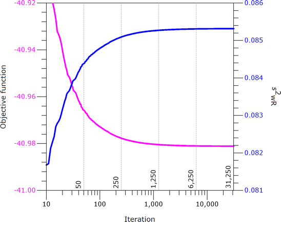
Fig. 9
REML: Iteration
history with FA0(2).
Failed to converge in allocated number of iterations. Output is suspect. Negative final variance component. Consider omitting this VC structure.
Note that \(\small{s_\text{wR}^2}\)
increases with the number of iterations, which is over-compensated by
increasing degrees of freedom and hence, the
CI narrows.
Note also that SAS forces negative variance components to
zero – which is questionable as well.
However, with CS (compound-symmetry) convergence was
achieved after just four [sic] iterations without any warnings:
\(\small{s_\text{wR}^2=0.089804}\),
\(\small{df=22.32592}\), \(\small{\text{90% CI}=\text{82.258 --
111.023}}\).
Welcome to the hell of mixed-effects modeling. Now I understand why Health Canada requires that the optimizer’s constraints are stated in the SAP.26
If you wonder whether a 3-period full replicate design is acceptable for agencies:
According to the EMA it is indeed.27
Already in 2001 the FDA recommended the 2-sequence 4-period full replicate design TRTR|RTRT but stated also:18
»Other replicated crossover designs are possible.
For example, a three-period design TRT|RTR could be used.
[…] the two-sequence, three-period design TRR|RTT is thought
to be optimal among three-period replicated crossover designs.«The guidance is in force for 23 years and the lousy partial replicate is not mentioned at all…
It is unclear whether the problematic 3-sequence partial replicate design mentioned more recently14 15 is mandatory or just given as an example. Does the overarching guidance about statistics in bioequivalence18 (which is final) overrule later ones, which are only drafts? If in doubt, initiate a ‘Controlled Correspondence’28 beforehand. Good luck!29
top of section ↩︎ previous section ↩︎
Study costs
Power (and hence, the sample size) depends on the number of
treatments – the smaller sample size in replicate designs is compensated
by more administrations. For
ABE costs of a replicate
design are similar to the common 2×2×2 crossover design. If the sample
size of a 2×2×2 design is n, then the sample size for a
4-period replicate design is ½ n and for a 3-period replicate
design ¾ n.
Nevertheless, smaller sample sizes come with a price. We have the same
number of samples to analyze and study costs are driven to a good part
by bioanalytics.30 We will save costs due to less
pre-/post-study exams but have to pay a higher subject remuneration
(more hospitalizations and blood samples). If applicable (depending on
the drug): Increased costs for in-study safety and/or
PD measurements.
Furthermore, one must be aware that more periods / washout phases
increase the chance of dropouts.
Let’s compare study costs (approximated by the number of treatments) of 3-period replicate designs to 4-period replicate designs planned for ABEL and RSABE. I assumed a T/R-ratio of 0.90, a CV-range of 30 – 65%, and targeted ≥ 80% power.
CV      <- seq(0.30, 0.65, 0.05)
theta0  <- 0.90
target  <- 0.80
designs <- c("2x2x4", "2x2x3", "2x3x3")
res1    <- data.frame(design = designs,
                      CV = rep(CV, each = length(designs)),
                      n = NA_integer_, n.trt = NA_integer_,
                      costs = "100% * ")
for (i in 1:nrow(res1)) {
  res1$n[i]     <- sampleN.scABEL(CV = res1$CV[i], theta0 = theta0,
                                  targetpower = target,
                                  design = res1$design[i],
                                  print = FALSE,
                                  details = FALSE)[["Sample size"]]
  n.per         <- as.integer(substr(res1$design[i], 5, 5))
  res1$n.trt[i] <- n.per * res1$n[i]
}
ref1 <- res1[res1$design == "2x2x4", c(1:2, 4)]
for (i in 1:nrow(res1)) {
  if (!res1$design[i] %in% ref1$design) {
    res1$costs[i] <- sprintf("%.0f%%   ", 100 * res1$n.trt[i] /
                                          ref1$n.trt[ref1$CV == res1$CV[i]])
  }
}
names(res1)[4:5] <- c("treatments", "rel. costs")
cat("ABEL (EMA and others)\n")
print(res1, row.names = FALSE)
# ABEL (EMA and others)
# design CV n treatments rel. costs
# 2x2x4 0.30 34 136 100% *
# 2x2x3 0.30 50 150 110%
# 2x3x3 0.30 54 162 119%
# 2x2x4 0.35 34 136 100% *
# 2x2x3 0.35 50 150 110%
# 2x3x3 0.35 48 144 106%
# 2x2x4 0.40 30 120 100% *
# 2x2x3 0.40 46 138 115%
# 2x3x3 0.40 42 126 105%
# 2x2x4 0.45 28 112 100% *
# 2x2x3 0.45 42 126 112%
# 2x3x3 0.45 39 117 104%
# 2x2x4 0.50 28 112 100% *
# 2x2x3 0.50 42 126 112%
# 2x3x3 0.50 39 117 104%
# 2x2x4 0.55 30 120 100% *
# 2x2x3 0.55 44 132 110%
# 2x3x3 0.55 42 126 105%
# 2x2x4 0.60 32 128 100% *
# 2x2x3 0.60 48 144 112%
# 2x3x3 0.60 48 144 112%
# 2x2x4 0.65 36 144 100% *
# 2x2x3 0.65 54 162 112%
# 2x3x3 0.65 54 162 112%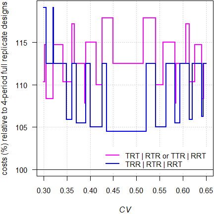
Fig. 10 ABEL: Relative costs of 3-period designs compared to 4-period full replicate designs.
In any case 3-period designs are more costly than 4-period full replicate designs. However, in the latter dropouts are more likely and the sample size has to be adjusted accordingly. Given that, the difference diminishes. Since there are no convergence issues in ABEL, the partial replicate can be used.
However, I prefer one of the 3-period full replicate designs due to the additional information about \(\small{CV_\text{wT}}\).
CV      <- seq(0.30, 0.65, 0.05)
theta0  <- 0.90
target  <- 0.80
designs <- c("2x2x4", "2x2x3", "2x3x3")
res2    <- data.frame(design = designs,
                      CV = rep(CV, each = length(designs)),
                      n = NA_integer_, n.trt = NA_integer_,
                      costs = "100% * ")
for (i in 1:nrow(res1)) {
  res2$n[i]     <- sampleN.RSABE(CV = res2$CV[i], theta0 = theta0,
                                 targetpower = target,
                                 design = res2$design[i],
                                 print = FALSE,
                                 details = FALSE)[["Sample size"]]
  n.per         <- as.integer(substr(res1$design[i], 5, 5))
  res2$n.trt[i] <- n.per * res2$n[i]
}
ref2 <- res2[res2$design == "2x2x4", c(1:2, 4)]
for (i in 1:nrow(res1)) {
  if (!res2$design[i] %in% ref2$design) {
    res2$costs[i] <- sprintf("%.0f%%   ", 100 * res2$n.trt[i] /
                                          ref2$n.trt[ref2$CV == res2$CV[i]])
  }
}
names(res2)[4:5] <- c("treatments", "rel. costs")
cat("RSABE (U.S. FDA and China CDE)\n")
print(res2, row.names = FALSE)
# RSABE (U.S. FDA and China CDE)
# design CV n treatments rel. costs
# 2x2x4 0.30 32 128 100% *
# 2x2x3 0.30 46 138 108%
# 2x3x3 0.30 45 135 105%
# 2x2x4 0.35 28 112 100% *
# 2x2x3 0.35 42 126 112%
# 2x3x3 0.35 39 117 104%
# 2x2x4 0.40 24 96 100% *
# 2x2x3 0.40 38 114 119%
# 2x3x3 0.40 33 99 103%
# 2x2x4 0.45 24 96 100% *
# 2x2x3 0.45 36 108 112%
# 2x3x3 0.45 33 99 103%
# 2x2x4 0.50 22 88 100% *
# 2x2x3 0.50 34 102 116%
# 2x3x3 0.50 30 90 102%
# 2x2x4 0.55 22 88 100% *
# 2x2x3 0.55 34 102 116%
# 2x3x3 0.55 30 90 102%
# 2x2x4 0.60 24 96 100% *
# 2x2x3 0.60 36 108 112%
# 2x3x3 0.60 33 99 103%
# 2x2x4 0.65 24 96 100% *
# 2x2x3 0.65 36 108 112%
# 2x3x3 0.65 33 99 103%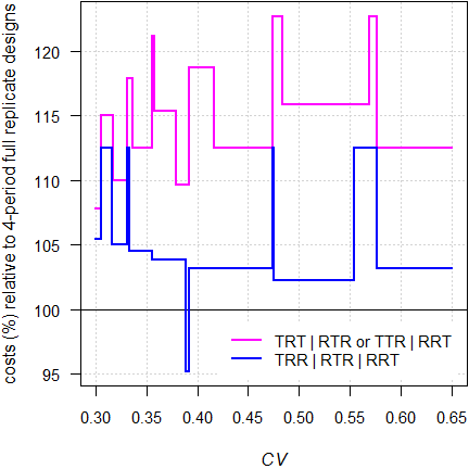
Fig. 11 RSABE: Relative costs of 3-period designs compared to 4-period full replicate designs.
In almost all cases 3-period designs are more costly than 4-period full replicate designs. However, in the latter dropouts are more likely and the sample size has to be adjusted accordingly. Given that, the difference diminishes. Due to the convergence issues in ABE (mandatory, if the realized \(\small{s_\text{wR}<0.294}\)), I strongly recommend to avoid the partial replicate design and opt for one of the 3-period full replicate designs instead.
Pros and Cons
From a statistical perspective, replicate designs are preferrable over the 2×2×2 crossover design. If we observe discordant31 outliers in the latter, we cannot distinguish between lack of compliance (the subject didn’t take the drug), a product failure, and a subject-by-formulation interaction (the subject belongs to a subpopulation).
A member of the EMA’s PKWP once told me that he would like to see all studies performed in a replicate design – regardless whether the drug / drug product is highly variable or not. One of the rare cases where we were of the same opinion.32
We design studies always for the worst case combination, i.e., based on the PK metric requiring the largest sample size. In jurisdictions accepting reference-scaling only for Cmax (e.g. by ABEL) the sample size is driven by AUC.
metrics <- c("Cmax", "AUCt", "AUCinf")
alpha   <- 0.05
CV      <- c(0.45, 0.34, 0.36)
theta0  <- rep(0.90, 3)
theta1  <- 0.80
theta2  <- 1 / theta1
target  <- 0.80
design  <- "2x2x4"
plan    <- data.frame(metric = metrics,
                      method = c("ABEL", "ABE", "ABE"),
                      CV = CV, theta0 = theta0,
                      L = 100*theta1, U = 100*theta2,
                      n = NA, power = NA)
for (i in 1:nrow(plan)) {
  if (plan$method[i] == "ABEL") {
    plan[i, 5:6] <- round(100*scABEL(CV = CV[i]), 2)
    plan[i, 7:8] <- signif(
                      sampleN.scABEL(alpha = alpha,
                                     CV = CV[i],
                                     theta0 = theta0[i],
                                     theta1 = theta1,
                                     theta2 = theta2,
                                     targetpower = target,
                                     design = design,
                                     details = FALSE,
                                     print = FALSE)[8:9], 4)
}else {
    plan[i, 7:8] <- signif(
                      sampleN.TOST(alpha = alpha,
                                   CV = CV[i],
                                   theta0 = theta0[i],
                                   theta1 = theta1,
                                   theta2 = theta2,
                                   targetpower = target,
                                   design = design,
                                   print = FALSE)[7:8], 4)
  }
}
txt <- paste0("Sample size based on ",
              plan$metric[plan$n == max(plan$n)], ".\n")
print(plan, row.names = FALSE)
cat(txt)
# metric method CV theta0 L U n power
# Cmax ABEL 0.45 0.9 72.15 138.59 28 0.8112
# AUCt ABE 0.34 0.9 80.00 125.00 50 0.8055
# AUCinf ABE 0.36 0.9 80.00 125.00 56 0.8077
# Sample size based on AUCinf.That’s outright bizarre (see also the article about post hoc power).
As special case is Health Canada, which accepts ABEL only for AUC, whereas for Cmax ABE has to be assessed for the conventional limits of 80.0–125.0%.
metrics <- c("Cmax", "AUCt", "AUCinf")
alpha   <- 0.05
CV      <- c(0.45, 0.34, 0.36)
theta0  <- rep(0.90, 3)
theta1  <- 0.80
theta2  <- 1 / theta1
target  <- 0.80
design  <- "2x2x4"
plan    <- data.frame(metric = metrics,
                      method = c("ABE", "ABEL", "ABEL"),
                      CV = CV, theta0 = theta0,
                      L = 100*theta1, U = 100*theta2,
                      n = NA, power = NA)
for (i in 1:nrow(plan)) {
  if (plan$method[i] == "ABEL") {
    plan[i, 5:6] <- round(100*scABEL(CV = CV[i]), 2)
    plan[i, 7:8] <- signif(
                      sampleN.scABEL(alpha = alpha,
                                     CV = CV[i],
                                     theta0 = theta0[i],
                                     theta1 = theta1,
                                     theta2 = theta2,
                                     targetpower = target,
                                     design = design,
                                     regulator = "HC",
                                     details = FALSE,
                                     print = FALSE)[8:9], 4)
}else {
    plan[i, 7:8] <- signif(
                      sampleN.TOST(alpha = alpha,
                                   CV = CV[i],
                                   theta0 = theta0[i],
                                   theta1 = theta1,
                                   theta2 = theta2,
                                   targetpower = target,
                                   design = design,
                                   print = FALSE)[7:8], 4)
  }
}
txt <- paste0("Sample size based on ",
              plan$metric[plan$n == max(plan$n)], ".\n")
print(plan, row.names = FALSE)
cat(txt)
# metric method CV theta0 L U n power
# Cmax ABE 0.45 0.9 80.00 125.00 84 0.8057
# AUCt ABEL 0.34 0.9 77.77 128.58 36 0.8123
# AUCinf ABEL 0.36 0.9 76.70 130.38 34 0.8040
# Sample size based on Cmax.As shown in the article about ABEL, we get an incentive in the sample size if \(\small{CV_\text{wT}<CV_\text{wR}}\). However, this does not help if reference-scaling is not acceptable (say, for the AUC in most jurisdictions) because the conventional model for ABE assumes homoscedasticity (\(\small{CV_\text{wT}\equiv CV_\text{wR}}\)).
theta0        <- 0.90
design        <- "2x2x4"
CVw           <- 0.36 # AUC - no reference-scaling
# variance-ratio 0.80: T lower than R
CV            <- signif(CVp2CV(CV = CVw, ratio = 0.80), 5)
# 'switch off' all scaling conditions of ABEL
reg           <- reg_const("USER", r_const = 0.76,
                           CVswitch = Inf, CVcap = Inf)
reg$pe_constr <- FALSE
res           <- data.frame(variance = c("homoscedastic", "heteroscedastic"),
                            CVwT = c(CVw, CV[1]), CVwR = c(CVw, CV[2]),
                            CVw = rep(CVw, 2), n = NA)
res$n[1]      <- sampleN.TOST(CV = CVw, theta0 = theta0,
                              design = design,
                              print = FALSE)[["Sample size"]]
res$n[2]      <- sampleN.scABEL(CV = CV, theta0 = theta0,
                                design = design, regulator = reg,
                                details = FALSE,
                                print = FALSE)[["Sample size"]]
print(res, row.names = FALSE)
# variance CVwT CVwR CVw n
# homoscedastic 0.36000 0.36000 0.36 56
# heteroscedastic 0.33824 0.38079 0.36 56Although we know that the test has a lower within-subject \(\small{CV}\) than the reference, this information is ignored and the (pooled) within-subject \(\small{CV_\text{w}}\) used.
Pros
- Statistically sound. Estimation of CVwR (and in full replicate designs additionally of CVwT) is possible. The additional information is a welcomed side effect.
- Mandatory for ABEL and RSABE. Smaller sample sizes than for ABE.
- ‘Outliers’ can be better assessed than in the 2×2×2 crossover
design.
- In the 2×2×2 crossover this will be rather difficult (exclusion of subjects based on statistical and/or PK grounds alone is not acceptable).
- For ABEL assessment of ‘outliers’ (of the reference treatment only) is part of the recommended procedure.33
Cons
- A larger sample size adjustment according to the anticipated dropout-rate required than in a 2×2×2 crossover design due to three or four periods instead of two.34
- Contrary to ABE – where
the limits are based on Δ according
to (1) – in practice the scaled limits of
SABE (2) are
calculated based on the realized swR.
- Without access to the study report, Δ cannot be re-calculated. This is an unsatisfactory situation for physicians, pharmacists, and patients alike.
- The elephant in the room: Potential inflation of the Type I Error (patient’s risk) in RSABE (if CVwR < 30%) and in ABEL (if ~25% < CVwR < ~42%). This issue is covered in another article.
Uncertain CVwR
An intriguing statement of the EMA’s Pharmacokinetics Working Party.
“Suitability of a 3-period replicate design scheme forI fail to find a statement in the guideline36 that \(\small{CV_\text{wR}}\) is a ‘key parameter’ – only that
the demonstration of within-subject variability for Cmax
The question raised asks if it is possible to use a design where subjects are randomised to receive treatments in the order of TRT or RTR. This design is not considered optimal […]. However, it would provide an estimate of the within subject variability for both test and reference products. As this estimate is only based on half of the subjects in the study the uncertainty associated with it is higher than if a RRT/RTR/TRR design is used and therefore there is a greater chance of incorrectly concluding a reference product is highly variable if such a design is used.
The CHMP bioequivalence guideline requires that at least 12 patients are needed to provide data for a bioequivalence study to be considered valid, and to estimate all the key parameters. Therefore, if a 3-period replicate design, where treatments are given in the order TRT or RTR, is to be used to justify widening of a confidence interval for Cmax then it is considered that at least 12 patients would need to provide data from the RTR arm. This implies a study with at least 24 patients in total would be required if equal number of subjects are allocated to the 2 treatment sequences.
»The number of evaluable subjects in a bioequivalence study should not be less than 12.«
However, in sufficiently powered studies such a situation is extremely unlikely (dropout-rate ≥ 42%).37
Let’s explore the uncertainty of \(\small{CV_\text{wR}=30\%}\) based on its 95% confidence interval in two scenarios:
- No dropouts. In the partial replicate design all subjects provide
data for the estimation of CVwR. In full
replicate designs only half of the subjects provide this
information.
- Extreme dropout-rates. Only twelve subjects remain in R-replicated sequence(s).
# CI of the CV for sample sizes of replicate designs
# (theta0 0.90, target power 0.80)
CV   <- 0.30
des  <- c("2x3x3", # 3-sequence 3-period (partial) replicate design
          "2x2x3", # 2-sequence 3-period full replicate designs
          "2x2x4") # 2-sequence 4-period full replicate designs
type <-c("partial", rep("full", 2))
seqs <- c("TRR|RTR|RTR",
          "TRT|RTR    ",
          "TRTR|RTRT  ")
res  <- data.frame(scenario = c(rep(1, 3), rep(2, 3)),
                   design = rep(des, 2), type = rep(type, 2),
                   sequences = rep(seqs, 2),
                   n = c(rep(NA, 3), rep(0, 3)),
                   RR = c(rep(NA, 3), rep(0, 3)), df = NA,
                   lower = NA, upper = NA, width = NA)
for (i in 1:nrow(res)) {
  if (is.na(res$n[i])) {
    res$n[i] <- sampleN.scABEL(CV = CV, design = res$design[i],
                               details = FALSE, print = FALSE)[["Sample size"]]
    if (res$design[i] == "2x2x3") {
      res$RR[i] <- res$n[i] / 2
  }else {
      res$RR[i] <- res$n[i]
    }
  }
  if (i > 3) {
    if (res$design[i] == "2x3x3") {
      res$n[i]  <- res$n[i-3] - 12
      res$RR[i] <- 12       # only 12 eligible subjects in sequence RTR
  }else {
      res$n[i]  <- 12       # min. sample size
      res$RR[i] <- res$n[i] # CVwR can be estimated
    }
  }
  res$df[i]   <- res$RR[i] - 2
  res[i, 8:9] <- CVCL(CV = CV, df = res$df[i],
                      side = "2-sided", alpha = 0.05)
  res[i, 10]  <- res[i, 9] - res[i, 8]
}
res[, 1]  <- sprintf("%.0f.", res[, 1])
res[, 8]  <- sprintf("%.1f%%", 100 * res[, 8])
res[, 9]  <- sprintf("%.1f%%", 100 * res[, 9])
res[, 10] <- sprintf("%.1f%%", 100 * res[, 10])
names(res)[1] <- ""
# Rows 1-2: Sample sizes for target power
# Rows 3-4: Only 12 eligible subjects to estimate CVwR
print(res, row.names = FALSE)
# design type sequences n RR df lower upper width
# 1. 2x3x3 partial TRR|RTR|RTR 54 54 52 25.0% 37.6% 12.5%
# 1. 2x2x3 full TRT|RTR 50 25 23 23.1% 43.0% 19.9%
# 1. 2x2x4 full TRTR|RTRT 34 34 32 23.9% 40.3% 16.4%
# 2. 2x3x3 partial TRR|RTR|RTR 42 12 10 20.7% 55.1% 34.4%
# 2. 2x2x3 full TRT|RTR 12 12 10 20.7% 55.1% 34.4%
# 2. 2x2x4 full TRTR|RTRT 12 12 10 20.7% 55.1% 34.4%Given, the CI of the \(\small{CV_\text{wR}}\) in the partial replicate design is narrower than in a three period full replicate design. Is that really relevant, esp. since only twelve eligible subjects in the RTR-sequence are acceptable to provide a ‘valid’ estimate?
Obviously the EMA’s
PKWP is aware of the
uncertainty of the realized \(\small{CV_\text{wR}}\), which may lead to a
misclassification (the study is assessed by
ABEL
although the drug / drug product is not highly variable) and
hence, a potentially inflated Type I Error (TIE, patient’s
risk). The partial replicate has – given studies with the same power –
the largest degrees of freedom and hence, leads to the lowest
TIE.38 However, it does not magically
disappear.
Such a misclassification may also affect the Type II Error (producer’s
risk). If the realized \(\small{CV_\text{wR}}\) is lower than
assumed in sample size estimation, less expansion can be applied and the
study will be underpowered. Of course, that’s not a regulatory
concern.
design  <- "2x2x4"
theta0  <- 0.90                  # asumed T/R-atio
CV.ass  <- 0.35                  # assumed CV
CV.real <- c(CV.ass, 0.30, 0.40) # realized CV
# sample size based on assumed T/R-ratio and CV, targeted at ≥ 80% power
res     <- data.frame(CV.ass = CV.ass,
                      n = sampleN.scABEL(CV = CV.ass, design = design,
                                         theta0 = theta0, details = FALSE,
                                         print = FALSE)[["Sample size"]],
                      CV.real = CV.real, L = NA_real_, U = NA_real_,
                      TIE = NA_real_, TIIE = NA_real_)
for (i in 1:nrow(res)) {
  res$L[i]    <- scABEL(CV = res$CV.real[i])[["lower"]]
  res$U[i]    <- scABEL(CV = res$CV.real[i])[["upper"]]
  res$TIE[i]  <- power.scABEL(CV = res$CV.real[i], design = design,
                              theta0 = res$U[i], n = res$n[i])
  res$TIIE[i] <- 1 - power.scABEL(CV = res$CV.real[i], design = design,
                                  theta0 = theta0, n = res$n[i])
}
res$CV.ass  <- sprintf("%.0f%%", 100 * res$CV.ass)
res$CV.real <- sprintf("%.0f%%", 100 * res$CV.real)
res$L       <- sprintf("%.2f%%", 100 * res$L)
res$U       <- sprintf("%.2f%%", 100 * res$U)
res$TIE     <- sprintf("%.5f", res$TIE)
res$TIIE    <- sprintf("%.4f", res$TIIE)
names(res)[c(1, 3)] <- c("assumed", "realized")
print(res, row.names = FALSE)
# assumed n realized L U TIE TIIE
# 35% 34 35% 77.23% 129.48% 0.06557 0.1882
# 35% 34 30% 80.00% 125.00% 0.08163 0.1972
# 35% 34 40% 74.62% 134.02% 0.05846 0.1535I recommend the article about power analysis (sections ABEL and RSABE).
Of note, if there are no / few dropouts, the estimated \(\small{CV_\text{wR}}\) in 4-period full replicate designs carries a larger uncertainty due to its lower sample size and therefore, less degrees of freedom. If the PKWP is concerned about an ‘uncertain’ estimate, why is this design given as an example?17 39 Many studies are performed in this design and are accepted by agencies.
Since for RSABE generally smaller sample sizes are required than for ABEL, the estimated \(\small{CV_\text{wR}}\) is more uncertain in the former.
# Cave: very long runtime
theta0 <- 0.90
target <- 0.80
CV     <- seq(0.3, 0.5, 0.00025)
x      <- seq(0.3, 0.5, 0.05)
des    <- c("2x3x3", # 3-sequence 3-period (partial) replicate design
            "2x2x3", # 2-sequence 3-period full replicate designs
            "2x2x4") # 2-sequence 4-period full replicate designs
RSABE  <- ABEL <- data.frame(design = rep(des, each = length(CV)),
                             n = NA, RR = NA, df = NA, CV = CV,
                             lower = NA, upper = NA)
for (i in 1:nrow(ABEL)) {
  RSABE$n[i] <- sampleN.RSABE(CV = RSABE$CV[i], theta0 = theta0,
                              targetpower = target,
                              design = RSABE$design[i],
                              details = FALSE,
                              print = FALSE)[["Sample size"]]
  if (RSABE$design[i] == "2x2x3") {
    RSABE$RR[i] <- RSABE$n[i] / 2
}else {
    RSABE$RR[i] <- RSABE$n[i]
  }
  RSABE$df[i]   <- RSABE$RR[i] - 2
  RSABE[i, 6:7] <- CVCL(CV = RSABE$CV[i], df = RSABE$df[i],
                        side = "2-sided", alpha = 0.05)
  ABEL$n[i]     <- sampleN.scABEL(CV = ABEL$CV[i], theta0 = theta0,
                                  targetpower = target,
                                  design = ABEL$design[i],
                                  details = FALSE,
                                  print = FALSE)[["Sample size"]]
  if (ABEL$design[i] == "2x2x3") {
    ABEL$RR[i] <- ABEL$n[i] / 2
}else {
    ABEL$RR[i] <- ABEL$n[i]
  }
  ABEL$df[i]   <- ABEL$RR[i] - 2
  ABEL[i, 6:7] <- CVCL(CV = ABEL$CV[i], df = ABEL$df[i],
                       side = "2-sided", alpha = 0.05)
}
ylim <- range(c(RSABE[6:7], ABEL[6:7]))
col  <- c("blue", "red", "magenta")
leg  <- c("2×3×3 (partial)", "2×2×3 (full)", "2×2×4 (full)")
dev.new(width = 4.5, height = 4.5, record = TRUE)
op   <- par(no.readonly = TRUE)
par(mar = c(4, 4.1, 0.2, 0.1), cex.axis = 0.9)
plot(CV, rep(0.3, length(CV)), type = "n", ylim = ylim, log = "xy",
     xlab = expression(italic(CV)[wR]),
     ylab = expression(italic(CV)[wR]*"  (95% confidence interval)"),
     axes = FALSE)
grid()
abline(h = 0.3, col = "lightgrey", lty = 3)
axis(1, at = x)
axis(2, las = 1)
axis(2, at = c(0.3, 0.5), las = 1)
lines(CV, CV, col = "darkgrey")
legend("topleft", bg = "white", box.lty = 0, title = "replicate designs",
       legend = leg, col = col, lwd = 2, seg.len = 2.5, cex = 0.9,
       y.intersp = 1.25)
box()
for (i in seq_along(des)) {
  lines(CV, RSABE$lower[RSABE$design == des[i]], col = col[i], lwd = 2)
  lines(CV, RSABE$upper[RSABE$design == des[i]], col = col[i], lwd = 2)
  y <- RSABE$upper[signif(RSABE$CV, 4) %in% x & RSABE$design == des[i]]
  n <- RSABE$n[signif(RSABE$CV, 4) %in% x & RSABE$design == des[i]]
  # sample sizes at CV = x
  shadowtext(x, y, labels = n, bg = "white", col = "black", cex = 0.75)
}
plot(CV, rep(0.3, length(CV)), type = "n", ylim = ylim, log = "xy",
     xlab = expression(italic(CV)[wR]),
     ylab = expression(italic(CV)[wR]*"  (95% confidence interval)"),
     axes = FALSE)
grid()
abline(h = 0.3, col = "lightgrey", lty = 3)
axis(1, at = x)
axis(2, las = 1)
axis(2, at = c(0.3, 0.5), las = 1); box()
lines(CV, CV, col = "darkgrey")
legend("topleft", bg = "white", box.lty = 0, title = "replicate designs",
       legend = leg, col = col, lwd = 2, seg.len = 2.5, cex = 0.9,
       y.intersp = 1.25)
box()
for (i in seq_along(des)) {
  lines(CV, ABEL$lower[ABEL$design == des[i]], col = col[i], lwd = 2)
  lines(CV, ABEL$upper[ABEL$design == des[i]], col = col[i], lwd = 2)
  y <- ABEL$upper[signif(ABEL$CV, 4) %in% x & ABEL$design == des[i]]
  n <- ABEL$n[signif(ABEL$CV, 4) %in% x & ABEL$design == des[i]]
  # sample sizes at CV = x
  shadowtext(x, y, labels = n, bg = "white", col = "black", cex = 0.75)
}
par(op)
cat("RSABE\n"); print(RSABE[signif(RSABE$CV, 4) %in% x, ], row.names = FALSE)
cat("ABEL\n"); print(ABEL[signif(ABEL$CV, 4) %in% x, ], row.names = FALSE)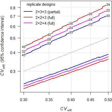
Fig. 11 RSABE (sample sizes for assumed T/R-ratio 0.90 targeted at ≥ 80% power).
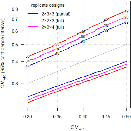
Fig. 12 ABEL (sample sizes for assumed T/R-ratio 0.90 targeted at ≥ 80% power).
That’s interesting. Say, we assumed \(\small{CV_\text{wR}=37\%}\), a T/R-ratio
0.90 targeted at ≥ 80% power in a 4-period full replicate design
intended for
ABEL.
We performed the study with 32 subjects. The 95%
CI of the \(\small{CV_\text{wR}}\) is 29.2% (no
expansion, assessment for
ABE) to 50.8% (already above
the upper cap of 50%).
Disturbing, isn’t it?
If you wonder why the confidence intervals are asymmetric (\(\small{CL_\text{upper}-CV_\text{wR}>CV_\text{wR}-CL_\text{lower}}\)): The \(\small{100\,(1-\alpha)}\) confidence interval of the \(\small{CV_\text{wR}}\) is obtained via the \(\small{\chi^2}\)-distribution of its error variance \(\small{s_\text{wR}^2}\) with \(\small{n-2}\) degrees of freedom. \[\begin{matrix}\tag{3} s_\text{wR}^2=\log_{e}(CV_\text{wR}+1)\\ L=\frac{(n-1)\,s_\text{wR}^2}{\chi_{\alpha/2,\,n-2}^{2}}\leq s_\text{wR}^2\leq\frac{(n-1)\,s_\text{wR}^2}{\chi_{1-\alpha/2,\,n-2}^{2}}=U\\ \left\{CL_\text{lower},\;CL_\text{upper}\right\}=\left\{\sqrt{\exp(L)-1},\sqrt{\exp(U)-1}\right\} \end{matrix}\]
The \(\small{\chi^2}\)-distribution
is skewed to the
right. Since the width of the confidence interval for a given \(\small{CV_\text{wR}}\) depends on the
degrees of freedom, it implies a more precise estimate in larger
studies, which will be required for relatively low variabilities (least
scaling).
In the example above the width of the
CI in the partial replicate
design is for
RSABE 0.139
(n 45) at \(\small{CV_\text{wR}=0.30}\) and 0.322
(n 30) at \(\small{CV_\text{wR}=0.50}\). For
ABEL
the widths are 0.125 (n 54) and 0.273 (n 39).
Postscript
Regularly I’m asked whether it is possible to use an adaptive Two-Stage Design (TSD) for ABEL or RSABE.
Whereas for ABE it is possible in principle (no method for replicate designs is published so far – only for 2×2×2 crossovers40), for SABE the answer is no. Contrary to ABE, where power and the Type I Error can be calculated by analytical methods, in SABE we have to rely on simulations. We would have to find a suitable adjusted \(\small{\alpha}\) and demonstrate beforehand that the patient’s risk will be controlled.
For the implemented regulatory frameworks the sample size estimation requires 105 simulations to obtain a stable result (see here and there). Since the convergence of the empiric Type I Error is poor, we need 106 simulations. Combining that with a reasonably narrow grid of possible \(\small{n_1}\) / \(\small{CV_\text{wR}}\)-combinations,41 we end up with with 1013 – 1014 simulations. I don’t see how that can be done in the near future, unless one has access to a massively parallel supercomputer. I made a quick estimation for my fast workstation: ~60 years running 24/7…
A manuscript submitted in June 2023 to the AAPS Journal proposing a TSD for RSABE was not accepted in March 2024 because the authors failed to demonstrate control of the Type I Error. Incidentally I was one of the reviewers…
As outlined above, SABE is rather insensitive to the CV. Hence, the main advantage of TSDs over fixed sample designs in ABE (re-estimating the sample size based on the CV observed in the first stage) is simply not relevant. Fully adaptive methods for the 2×2×2 crossover allow also to adjust for the PE observed in the first stage. Here it is not possible. If you are concerned about the T/R-ratio, perform a (reasonably large!)42 pilot study and – even if the T/R-ratio looks promising – plan for a ‘worse’ one since it is not stable between studies.
top of section ↩︎ previous section ↩︎
Post postscript
Let’s recap the basic mass balance equation of PK: \[\small{F\cdot D=V\cdot k\,\cdot\int_{0}^{\infty}C(t)\,dt=CL\cdot AUC_{0-\infty}}\tag{4}\] We assess bioequivalence by comparative bioavailability,43 i.e., \[\small{\frac{F_{\text{T}}}{F_{\text{R}}}\approx \frac{AUC_{\text{T}}}{AUC_{\text{R}}}}\tag{5}\] That’s only part of the story because – based on \(\small{(4)}\) – actually \[\small{AUC_{\text{T}}=\frac{F_\text{T}\cdot D_\text{T}}{CL}\;\land\;AUC_{\text{R}}=\frac{F_\text{R}\cdot D_\text{R}}{CL}}\tag{6}\] Since an adjustment for measured potency is generally not acceptable, we have to assume that the true contents equal the declared ones and further \[\small{D_\text{T}\equiv D_\text{R}}\tag{7}\] This allows us to eliminate the doses from \(\small{(6)}\); however, we still have to assume no inter-occasion variability of clearances (\(\small{CL=\text{const}}\)) in order to arrive at \(\small{(5)}\).
Great, but is that true‽ If we have to deal with a HVD, the high variability is an intrinsic property of the drug itself (not the formulation). In BE were are interested in detecting potential differences of formulations, right? Since we ignored the – possibly unequal – clearances, all unexplained variability goes straight to the residual error, results in a large within-subject variance and hence, a wide confidence interval. In other words, the formulation is punished for a crime that clearance committed.
Can we do anything against it – apart from reference-scaling? We know that \[\small{k=CL\big{/}V}\tag{8}\] In crossover designs the volume of distribution of healthy subjects likely shows limited inter-occasion variability. Therefore, we can drop the volume of distribution and approximate the effect of \(\small{CL}\) by \(\small{k}\). This leads to \[\small{\frac{F_{\text{T}}}{F_{\text{R}}}\sim \frac{AUC_{\text{T}}\cdot k_{\text{T}}}{AUC_{\text{R}}\cdot k_{\text{R}}}}\tag{9}\] A variant of \(\small{(9)}\) – using \(\small{t_{1/2}}\)44 instead of \(\small{k}\) – was explored already in the dark ages.45 46
“Although there was wide variation in […] estimated halflife in these studies, the average area / dose × halflife ratios are amazingly similar. “[…] the assumption of constant clearance in the individual between the occasions of receiving the standard and the test dose is suspect for theophylline. […] If there is evidence that the clearance but not the volume of distribution varies in the individual, the AUC × k can be used to gain a more precise index of bioavailability than obtainable from AUC alone.
Confirmed (esp. for \(\small{AUC_{0-\infty}}\)) in the data set
Theoph48 which is part of the Base R installation: \[\small{\begin{array}{lc}
\text{PK metric} & CV_\text{geom}\,\%\\\hline
AUC_{0-\text{tlast}} & {\color{Red} {22.53\%}}\\
AUC_{0-\text{tlast}} \times k & {\color{Blue} {21.81\%}}\\
AUC_{0-\infty} & {\color{Red} {28.39\%}}\\
AUC_{0-\infty} \times k & {\color{Blue} {20.36\%}}\\\hline
\end{array}}\]
“Abstract
Aim: To quantify the utility of a terminal-phase adjusted area under the concentration curve method in increasing the probability of a correct and conclusive outcome of a bioequivalence (BE) trial for highly variable drugs when clearance (CL) varies more than the volume of distribution (V).
Methods: Data from a large population of subjects were generated with variability in CL and V, and used to simulate a two-period, two-sequence crossover BE trial. The 90% confidence interval for formulation comparison was determined following BE assessment using the area under the concentration curve (AUC) ratio test, and the proposed terminal-phase adjusted AUC ratio test. An outcome of bioequivalent, non-bioequivalent or inconclusive was then assigned according to predefined BE limits.
Results: When CL is more variable than V, the proposed approach would enhance the probability of correctly assigning bioequivalent or non-bioequivalent and reduce the risk of an inconclusive trial. For a hypothetical drug with between-subject variability of 35% for CL and 10% for V, when the true test-reference ratio of bioavailability is 1.15, a cross-over study of n=14 subjects analyzed by the proposed method would have 80% or 20% probability of claiming bioequivalent or non-bioequivalent, compared to 22%, 46% or 32% probability of claiming bioequivalent, non-bioequivalent or inconclusive using the standard AUC ratio test.
Conclusions: The terminal-phase adjusted AUC ratio test represents a simple and readily applicable approach to enhance the BE assessment of drug products when CL varies more than V.
I ❤ the idea. When Abdallah’s paper49 was published, I tried the approach retrospectively in a couple of my studies. It worked mostly, and if not, it was a HVDP, where the variability is caused by the formulation (e.g., gastric-resistant diclofenac).
That’s basic PK and \(\small{CL=\text{const}}\) is a rather strong assumption, which might be outright false. Consequently the whole concept of BE testing is built on sand: Studies are substantially larger than necessary, exposing innocent subjects to nasty drugs.
“It is recommended that area correction be attempted in bioequivalence studies of drugs where high intrasubject variability in clearance is known or suspected. […] The value of this approach in regulatory decision making remains to be determined. “Performance of the AUC·k ratio test […] indicate that the regulators should consider the method for its potential utility in assessing HVDs and lessening unnecessary drug exposure in BE trials.
For HVDs (not HVDPs) probably we could counteract the high variability, avoid the – potentially – inflated Type I Error in SABE (which is covered in another article), use conventional ABE with fixed limits,51 and all will be good. Perhaps the agencies should revise their guidelines. Hope dies last.
top of section ↩︎ previous section ↩︎
Licenses
 Helmut Schütz 2024
R and PowerTOST GPL 3.0,
TeachingDemos Artistic 2.0,
klippy MIT,
pandoc GPL 2.0.
1st version April 22, 2021. Rendered April 5, 2024 11:25 CEST
by rmarkdown
via pandoc in 0.37 seconds.
Footnotes and References
Labes D, Schütz H, Lang B. PowerTOST: Power and Sample Size for (Bio)Equivalence Studies. CRAN.↩︎
Snow G. TeachingDemos: Demonstrations for Teaching and Learning. Package version 2.13. 2024-02-16. CRAN.↩︎
Schütz H. Reference-Scaled Average Bioequivalence. 2022-02-19. CRAN.↩︎
Labes D, Schütz H, Lang B. Package PowerTOST’. February 21, 2022. CRAN.↩︎
Some gastric resistant formulations of diclofenac are HVDPs, practically all topical formulations are HVDPs, whereas diclofenac itself is not a HVD (\(\small{CV_\text{w}}\) of a solution ~8%).↩︎
An exception is dabigatran, the first univalent direct thrombin (IIa) inhibitor. The originator withheld information about severe bleeding events. Although dabigatran is highly variable, reference-scaling is not justified. The FDA requires for dabigatran, rivaroxaban, and edoxaban 4-period full replicate studies with the conventional limits and additionally comparing \(\small{s_\text{wT}}\) with \(\small{s_\text{wR}}\).↩︎
Note that the model of SABE is based on the true \(\small{\sigma_\text{wR}}\), whereas in practice the observed \(\small{s_\text{wR}}\) is used.↩︎
Note that the intention to apply one of the SABE-methods must be stated in the protocol. It is neither acceptable to switch post hoc from ABE to SABE nor between methods (say, from ABEL to the more permissive RSABE).↩︎
\(\small{CV_\text{wR}=100\sqrt{\exp(0.294^2)-1}=30.04689\ldots\%}\)↩︎
Health Canada, TPD. Notice: Policy on Bioequivalence Standards for Highly Variable Drug Products. Ottawa. April 18, 2016. Online.↩︎
Tóthfalusi L, Endrényi L. Sample Sizes for Designing Bioequivalence Studies for Highly Variable Drugs. J Pharm Pharmaceut Sci. 2012; 15(1): 73–84. doi:10.18433/J3Z88F.
 Open
Access.↩︎
Open
Access.↩︎Benet L. Why Highly Variable Drugs are Safer. Presentation at the FDA Advisory Committee for Pharmaceutical Science. Rockville. 06 October, 2006.
 Internet
Archive.↩︎
Internet
Archive.↩︎FDA, OGD. Draft Guidance on Progesterone. Rockville. Recommended April 2010, Revised February 2011. Download.↩︎
FDA, CDER. Draft Guidance. Bioequivalence Studies With Pharmacokinetic Endpoints for Drugs Submitted Under an ANDA. Silver Spring. August 2021. Download.↩︎
FDA, CDER. Guidance for Industry. Statistical Approaches to Establishing Bioequivalence. Rockville. January 2001. Download.↩︎
Fuglsang A. Mitigation of the convergence issues associated with semi-replicated bioequivalence data. Pharm Stat. 2021; 20(6): 1232–4. doi:10.1002/pst.2142.↩︎
SAS Institute Inc. SAS® 9.4 and SAS® Viya® 3.3 Programming Documentation. The MIXED Procedure. February 13, 2019. Online.↩︎
Balaam LN. A Two-Period Design with t2 Experimental Units. Biometrics. 1968; 24(1): 61–73. doi:10.2307/2528460.↩︎
Chow, SC, Shao J, Wang H. Individual bioequivalence testing under 2×3 designs. Stat Med. 2002; 21(5): 629–48. doi:10.1002/sim.1056.↩︎
Aka the ‘extra-reference’ design. It should be avoided because it is biased in the presence of period effects because T is not administered in the 3rd period.↩︎
FDA, CDER. ANDA Submissions – Refuse-to-Receive Standards. Silver Spring. Revision 2. December 2016 Download.↩︎
If you want to try it in your software: Download 20.5 MiB in CSV format.↩︎
Certara USA, Inc., Princeton, NJ. Phoenix® WinNonlin® version 8.1. 2018.↩︎
Health Canada, TPD. Guidance Document: Conduct and Analysis of Comparative Bioavailability Studies. Section 2.7.4.2 Model Fitting. Ottawa. 2018/06/08. Online.↩︎
EMA, CHMP. Questions & Answers: positions on specific questions addressed to the Pharmacokinetics Working Party (PKWP). Rev. 13. London. 19 November 2015. Online.↩︎
FDA, CDER. Guidance for Industry. Controlled Correspondence Related to Generic Drug Development. Silver Spring. December 2020. Download.↩︎
A member of the BEBA-Forum faced two partial replicate studies where softwares’ optimizer failed to converge (both SAS and Phoenix WinNonlin). Luckily, these were just pilot studies. He sent letters to the FDA requesting a clarification. He never received an answer.
At a webinar in March 2023 I tried to ask Donald Schuirmann. The 👨✈️steeringmoderating the »Panel Discussions« decided to ignore my question… Instead, the only question related to SABE was ‘How is a Highly Variable Drug defined?’, which Schuirmann explained at great length. Oh dear, what a waste of time!↩︎In case of a ‘poor’ bioanalytical method requiring a large sample volume: Since the total blood sampling volume is generally limited with the one of a blood donation, one may opt for a 3-period full replicate or has to measure hematocrit prior to administration in higher periods and – for safety reasons – exclude subjects if their HCT is too high.↩︎
The T/R-ratio in a particular subject differs from other subjects showing a ‘normal’ response. A concordant outlier will show deviant responses for both T and R. That’s not relevant in crossover designs.↩︎
If the study was planned for ABE, fails due to lacking power (\(\small{CV}\) higher than assumed and \(\small{CV_\text{wR}>30\%}\), and reference-scaling would be acceptable (no safety/efficacy issues with the expanded limits), one has already estimates of \(\small{CV_\text{wR}}\) and \(\small{CV_\text{wT}}\) and is able to design the next study properly.↩︎
The \(\small{CV_\text{wR}}\) has to be recalculated after exlusion of the outlier(s), leading to less expansion of the limits. Nevertheless, the outlying subject(s) has/have to be kept in the data set for calculating the 90% CI. However, that contradicts the principle »The data from all treated subjects should be treated equally« stated in the guideline. Oh dear!↩︎
Also two or three washout phases instead of one. Once we faced a case when during a washout a volunteer was bitten by a dog. I’m not kidding. Since he had to visit a hospital to get his wound sutured, according to the protocol it was rated as a – not drug-related – SAE and we had to exlude him from the study. Shit happens.↩︎
EMA. Questions & Answers: positions on specific questions addressed to the Pharmacokinetics Working Party (PKWP). London. June 2015 (Rev. 12 and later). Online.↩︎
EMA, CHMP. Guideline on the Investigation of Bioequivalence. London. 20 January 2010. Online.↩︎
Schütz H. The almighty oracle has spoken! BEBA Forum. Vienna. 2015-07-23. Online.↩︎
Labes D, Schütz H. Inflation of Type I Error in the Evaluation of Scaled Average Bioequivalence, and a Method for its Control. Pharm Res. 2016; 33(11): 2805–14. doi:10.1007/s11095-016-2006-1.↩︎
EMA. EMA/582648/2016. Annex II. London. 21 September 2016. Online.↩︎
Maurer W, Jones B, Chen Y. Controlling the type 1 error rate in two-stage sequential designs when testing for average bioequivalence. Stat Med. 2018; 37(10): 1587–1607. doi:10.1002/sim.7614.↩︎
Step sizes of \(\small{n_1}\) 2 in full replicate designs and 3 in the partial replicate design; step size of \(\small{CV_\text{wR}}\) 2%.↩︎
I know one large generic player’s rule for pilot studies of HVD(P)s: The minimum sample size is 24 in a four-period full replicate design. I have seen pilot studies with 80 [sic] subjects.↩︎
There are no ‘bioequivalence studies’! Bioequivalence is the desired result of a comparative bioavailability study. Only Health Canada gets it right in its guidances. Kudos!↩︎
Wagner JG. Method of Estimating Relative Absorption of a Drug in a Series of Clinical Studies in Which Blood Levels Are Measured After Single and/or Multiple Doses. J Pharm Sci. 1967; 56(5): 652–3. doi:10.1002/jps.2600560527.↩︎
Before the portmanteau word ‘bioavailability’ (of ‘biological’ and ‘availability’) was coined by Lindenbaum et al. in 1971. Try to search for earlier papers with the keyword ‘bioavailability’. You will be surprised.↩︎
Lindenbaum J, Mellow MH, Blackstone MO, Butler VP. Variation in Biologic Availability of Digoxin from Four Preparations. N Engl J Med. 1971; 285: 1344–7. doi:10.1056/nejm19711209285240.↩︎
Upton RA, Sansom L, Guentert TW, Powell JR, Thiercellin J-F, Shah VP, Coates PE, Riegelman S. Evaluation of the Absorption from 15 Commercial Theophylline Products Indicating Deficiencies in Currently Applied Bioavailability Criteria. J Pharmacokin Biopharm. 1980; 8(3): 229–42. doi:10.1007/BF01059644.↩︎
Study D, Treatment II of Upton et al.: Slophyllin aqueous syrup (Dooner Laboratories), 80 mg theophylline per 15-mL dose, 60 mL ≈ 320 mg administered, twelve subjects, sampling: 0, 0.25, 0.5, 1, 2, 3.5, 5, 7, 9, 12, and 24 hours. Linear-up / log-down trapezoidal rule, extrapolation based on \(\small{\widehat{C}_\text{last}}\) [sic].↩︎
Abdallah HY. An area correction method to reduce intrasubject variability in bioequivalence studies. J Pharm Pharmaceut Sci. 1998; 1(2): 60–5.
Open
Access.↩︎Lucas AJ, Ogungbenro K, Yang S, Aarons L. Chen C. Evaluation of area under the concentration curve adjusted by the terminal-phase as a metric to reduce the impact of variability in bioequivalence testing. Br J Clin Pharmacol. 2022; 88(2): 619–27. doi:10.1111/bcp.14986.↩︎
Schütz H, Labes D, Wolfsegger MJ. Critical Remarks on Reference-Scaled Average Bioequivalence. J Pharm Pharmaceut Sci. 2022; 25: 285–296. doi:10.18433/jpps32892.
Open
Access.↩︎