
Carryover
A Never Ending Story
Helmut Schütz
April 2, 2024
Consider allowing JavaScript. Otherwise, you have to be proficient in
reading  since formulas
will not be rendered. Furthermore, the table of contents in the left
column for navigation will not be available and code-folding not
supported. Sorry for the inconvenience.
since formulas
will not be rendered. Furthermore, the table of contents in the left
column for navigation will not be available and code-folding not
supported. Sorry for the inconvenience.
Examples in this article were generated with
 4.3.3 and the packages
 PowerTOST,1 nlme,2
lme4,3 and lmerTest.4
- The right-hand badges give the respective section’s ‘level’.
- Basics about assessment of (bio)equivalence trials – requiring no or only limited statistical expertise.
- These sections are the most important ones. They are – hopefully – easily comprehensible even for novices.
- A somewhat higher knowledge of statistics and/or R is required. May be skipped or reserved for a later reading.
- An advanced knowledge of statistics and/or R is required. Not recommended for beginners in particular.
- Click to show / hide R code.
- Click on the icon
 in the top left corner to copy R code to the
clipboard.
in the top left corner to copy R code to the
clipboard.
A basic knowledge of R does not
hurt. To run the simulation scripts at least version
1.4.3 (2016-11-01) of PowerTOST is suggested. Any version
of R would likely do, though the current
release of PowerTOST was only tested with version 4.2.3
(2023-03-15) and later. All scripts were run on a Xeon E3-1245v3 @
3.40GHz (1/4 cores) 16GB RAM with R 4.3.3 on
Windows 7 build 7601, Service Pack 1, Universal C Runtime
10.0.10240.16390.
Introduction
What is a significant sequence (carryover) effect and do we have to care about one?
I will try to clarify why such a ‘justification’ is not possible and – a bit provocative – asking for one demonstrates a lack of understanding the underlying statistical concepts.
All examples deal with the 2×2×2 crossover design (RT|TR)5 but are applicable to Higher-Order crossovers and replicate designs as well.
Carryover means that one treatment (R or T) administered in one period affects the PK response of the respective other treatment (T or R) administered in a subsequent period. If this is the case, the comparison of T vs R depends on the sequence of administrations and the result could be biased.
- If the sequence of administrations (RT or TR) does not affect the
PK response:
Carryover and the sequence effect are zero → the estimate is unbiased. - If the sequence of administrations (RT or TR) affects the
PK response to the same
extent:
Carryover is equal and the sequence effect zero → the estimate is unbiased. - If the sequence of administrations (RT or TR) affects the
PK response to a different
extent:
Carryover is unequal and the sequence effect ≠ zero → the estimate is unavoidably biased.
Since carryover cannot be extracted from the data, the bias is unknown.
The last case is of course problematic and makes the result of a crossover study questionable.
“The intuitive appeal of having each subject serve as his or her own control has made the crossover study one of the most popular experimental strategies since the infancy of formal experimental design. Frequent misapplications of the design in clinical experiments, and frequent misanalyses of the data, motivated the Biometric and Epidemiological Methodology Advisory Committee to the U.S. FDA to recommend in June of 1977 that, in effect, the crossover design be avoided in comparative clinical studies except in the rarest instances.
However, in bioequivalence crossover designs are the rule and parallel designs the exception.
Model
As the most simple case the 2×2×2 design (\(\small{\textrm{RT}|\textrm{TR}}\))
including a term for carryover is considered.7 Let sequences and
periods be indexed by \(\small{i}\) and
\(\small{k}\) (\(\small{i,k=1,2}\)) and \(\small{n_i}\) subjects are randomized to
sequence \(\small{i}\). Let \(\small{Y_{ijk}}\) be the \(\small{\log_{e}}\)-transformed
PK-response of the \(\small{j}\)th subject in the \(\small{i}\)th sequence at the \(\small{k}\)th period. Then \[Y_{ijk}=\mu_h+s_{ij}+\pi_k+\lambda_c+e_{ijk},\tag{1}\]
where \(\small{\mu_h}\) is effect of
treatment \(\small{h}\), where \(\small{h=\textrm{R}}\) if \(\small{i=k}\) and \(\small{h=\textrm{T}}\) if \(\small{i\neq k}\),
\(\small{s_{ij}}\) is the fixed effect
of the \(\small{j}\)th subject in the
\(\small{i}\)th sequence,
\(\small{\pi_{j}}\) is the fixed effect
of the \(\small{k}\)th period,
\(\small{\lambda_{c}}\) is the
carryover effect of the corresponding formulation from period 1 to
period 2, where
\(\small{c=\textrm{R}}\) if \(\small{i=1,k=2}\),
\(\small{c=\textrm{T}}\) if \(\small{i=2,k=2}\),
\(\small{\lambda_{c}=0}\) if
\(\small{i=1,2,k=1}\),
\(\small{e_{ijk}}\) is the random error
in observing \(\small{Y_{ijk}}\) (of
the \(\small{j}\)th subject in the
\(\small{k}\)th period and \(\small{i}\)th sequence).
The subject effects \(\small{s_{ij}}\) are independently8 normally distributed with expected mean \(\small{0}\) and between-subject variance \(\small{\sigma_{\textrm{b}}^{2}}\). The random errors \(\small{e_{ijk}}\) are independent and normally distributed with expected mean \(\small{0}\) and variances \(\small{\sigma_{\textrm{wR}}^{2}}\), \(\small{\sigma_{\textrm{wT}}^{2}}\) for the reference and test treatment. The treatment variances are given by \(\small{\sigma_{\textrm{R}}^{2}=\sigma_{\textrm{b}}^{2}+\sigma_{\textrm{wR}}^{2}}\) and \(\small{\sigma_{\textrm{T}}^{2}=\sigma_{\textrm{b}}^{2}+\sigma_{\textrm{wT}}^{2}}\). Note that these components cannot be separately estimated in a nonreplicative design.
Therefore, the layout of the \(\small{\textrm{RT}|\textrm{TR}}\) design is:
| Sequence | Period 1 | Period 2 |
|---|---|---|
| 1 (\(\small{\textrm{RT}}\)) |
\(\small{Y_{1j1}=\mu_\textrm{R}+s_{1j}+\pi_1+e_{1j1}}\) \(\small{j=1,\ldots,n_1}\) |
\(\small{Y_{1j2}=\mu_\textrm{T}+s_{1j}+\pi_2+\lambda_\textrm{R}+e_{1j2}}\) \(\small{j=1,\ldots,n_1}\) |
| 2 (\(\small{\textrm{TR}}\)) |
\(\small{Y_{2j1}=\mu_\textrm{T}+s_{2j}+\pi_1+e_{2j1}}\) \(\small{j=1,\ldots,n_2}\) |
\(\small{Y_{2j2}=\mu_\textrm{R}+s_{2j}+\pi_2+\lambda_\textrm{T}+e_{2j2}}\) \(\small{j=1,\ldots,n_2}\) |
The expected population means and variances are given by:
| Sequence | Period 1 | Period 2 |
|---|---|---|
| 1 (\(\small{\textrm{RT}}\)) |
\(\small{E(Y_{1j1})=\mu_\textrm{R}+\pi_1}\) \(\small{Var(Y_{1j1})=\sigma_{\textrm{R}}^{2}=\sigma_{\textrm{b}}^{2}+\sigma_{\textrm{wR}}^{2}}\) \(\small{j=1,\ldots,n_1}\) |
\(\small{E(Y_{1j2})=\mu_\textrm{T}+\pi_2+\lambda_\textrm{R}}\) \(\small{Var(Y_{1j2})=\sigma_{\textrm{T}}^{2}=\sigma_{\textrm{b}}^{2}+\sigma_{\textrm{wT}}^{2}}\) \(\small{j=1,\ldots,n_1}\) |
| 2 (\(\small{\textrm{TR}}\)) |
\(\small{E(Y_{2j1})=\mu_\textrm{T}+\pi_1}\) \(\small{Var(Y_{2j1})=\sigma_{\textrm{T}}^{2}=\sigma_{\textrm{b}}^{2}+\sigma_{\textrm{wT}}^{2}}\) \(\small{j=1,\ldots,n_2}\) |
\(\small{E(Y_{2j2})=\mu_\textrm{R}+\pi_2+\lambda_\textrm{T}}\) \(\small{Var(Y_{2j2})=\sigma_{\textrm{R}}^{2}=\sigma_{\textrm{b}}^{2}+\sigma_{\textrm{wR}}^{2}}\) \(\small{j=1,\ldots,n_2}\) |
Assuming equal carryover (\(\small{\lambda_\textrm{R}=\lambda_\textrm{T}}\)), the term \(\small{\lambda_c}\) for carryover can be dropped from the model.
Implementation
“Ideally, all treated subjects should be included in the statistical analysis. However, subjects in a crossover trial who do not provide evaluable data for both of the test and reference products […] should not be included.
Most agencies (like the EMA) require an ANOVA of \(\small{\log_{e}}\) transformed responses, i.e., a linear model where all effects are fixed.
In R
model <- lm(log(PK) ~ sequence + subject %in% sequence +
                      period + treatment, data = data)
coef(model)[["treatmentT"]]
confint(model, "treatmentT", level = 0.9)SAS
PROC GLM
  data = data;
  class subject period sequence treatment;
  model logPK = sequence subject(sequence)
                period treatment;
  estimate 'T-R' treatment -1 1 / CL alpha = 0.1;
run;
In Phoenix WinNonlin
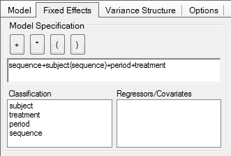
Note that in comparative bioavailability studies subjects are
generally uniquely coded.
If subject 1 is randomized to sequence RT,
there is not ‘another’ subject 1 randomized to sequence TR. Hence, the term subject(sequence) stated in all
guidelines is a bogus one. Actually it is an insult to the mind.
Replacing it with the simple term subject gives exactly [sic] the
same relevant results.
Doing so avoids the many lines in the output denoted with not estimable in Phoenix WinNonlin
and . in SAS.
Heresy: You could even drop sequence from the model entirely. That’s the model given by one of the pioneers of BE, Wilfred J. Westlake10 11 and I have used in hundreds of studies.
model <- lm(log(PK) ~ subject + period + treatment,
data = data)| Model | MSE | PE | 90% CI |
|---|---|---|---|
| 1 Nested: sequence + subject(sequence) | 0.05568 | 0.9541 | 0.8568 – 1.0625 |
| 2 Simple: sequence + subject | 0.05568 | 0.9541 | 0.8568 – 1.0625 |
| 3 Heretic: subject | 0.05568 | 0.9541 | 0.8568 – 1.0625 |
Quod erat demonstrandum. Sapienti sat! So much about over-parameterized models.
Other agencies (e.g., Health Canada) prefer a mixed-effects model, where \(\small{s_{ij}}\) is a random effect and all others fixed.
“By definition the cross-over design is a mixed effects model with fixed and random effects. The basic two period cross-over can be analysed according to a simple fixed effects model and least squares means estimation. Identical results will be obtained from a mixed effects analysis such as Proc Mixed in SAS®. If the mixed model approach is used, parameter constraints should be defined in the protocol.
In
SAS
PROC MIXED
  data = data;
  class subject period sequence treatment;
  model logPK = sequence subject(sequence)
                period treatment;
  estimate 'T-R' treatment -1 1 / CL alpha = 0.1;
run;
In Phoenix WinNonlin
Problems
Aliasing
The sequence effect is aliased (confounded) with
- the carryover effect and
- the treatment-by-period interaction.15
A statistically significant sequence effect could indicate that there is
- a true sequence effect, or
- a true treatment-by-period interaction, or
- a failure in randomization.
Only the last potential cause can be ruled out during monitoring or in an audit/inspection.
Wrong Test
To assess the sequence effect these tests are commonly used: \[\small{F=\frac{MSE_{\,\textrm{sequence}}}{MSE_{\,\textrm{residual}}}}\tag{2}\] \[\small{F=\frac{MSE_{\,\textrm{sequence}}}{MSE_{\,\textrm{subject(sequence)}}}}\tag{3}\] \[\small{F=\frac{MSE_{\,\textrm{sequence}}}{MSE_{\,\textrm{subject}}}}\tag{4}\]
The \(\small{p}\)-value of the tests is calculated by \[\small{p(F)=F_{\,\nu_1,\,\nu_2},}\tag{5}\] where \(\small{\nu_1}\) are the numerator’s degrees of freedom (\(\small{n_\textrm{seq}-1}\), where in a 2×2×2 crossover \(\small{\nu_1=1}\)) and \(\small{\nu_2}\) are the denominator’s degrees of freedom (in a 2×2×2 crossover \(\small{\nu_2=n_\textrm{RT}+n_\textrm{TR}-2}\)).
According to \(\small{(1)}\) carryover has the same levels as treatments and hence, the correct test has to be performed between subjects. Therefore, the Mean Squares Error of \(\small{\text{sequence}}\) has to be tested against the \(\small{MSE}\) of \(\small{\text{subject(sequence)}}\) in the nested model by \(\small{(3)}\)16 – or against the \(\small{MSE}\) of \(\small{\text{subject}}\) in the simple model by \(\small{(4)}\)17 – and not against the \(\small{\text{residual}}\) \(\small{MSE}\) by \(\small{(2)}\) – which is a within subject term.
Since generally \(\small{s_\textrm{w}^2<s_\textrm{b}^2}\), at test by \(\small{(2)}\) will be more often statistically significant than by \(\small{(3)}\) or \(\small{(4)}\).
\(\small{(2)}\)
is implemented in R’s function
anova()18 and obtained in the default ‘Partial SS’
of Phoenix WinNonlin,19 i.e., Type I20 effects
are estimated. In SAS21 – depending on its setup –
Type I by \(\small{(2)}\),
Type III by \(\small{(3)}\) or \(\small{(4)}\), or both are given in the
output.
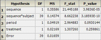
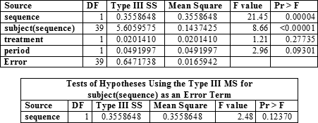
An example from my files (\(\small{n_\textrm{TR}=20,\;n_\textrm{RT}=21;\;n=41}\)): \[\small{\begin{array}{lrrrrrl} \text{Type I by (2)} & \nu & SSE & MSE & F & p(F)\\ \hline \text{sequence} & 1 & 0.355865 & 0.3558648 & 21.44519 & 3.9837\text{e-05} & \text{***}\\ \text{subject(sequence)} & 39 & 5.605958 & 0.1437425 & 8.66224 & 3.1856\text{e-10} & \text{***}\\ \text{period} & 1 & 0.049200 & 0.0491997 & 2.96488 & 0.093014 & \text{.}\\ \text{treatment} & 1 & 0.020141 & 0.0201405 & 1.21371 & 0.277351\\ \text{residuals} & 39 & 0.647172 & 0.0165942\\\hline \\ \text{Type III by (3)} & \nu & SSE & MSE & F & p(F)\\ \hline \text{sequence} & 1 & 0.355865 & 0.3558648 & 2.47571 & 0.123696\\ \text{subject(sequence)} & 39 & 5.605958 & 0.1437425 & 8.66224 & 3.1856\text{e-10} & \text{***}\\ \text{period} & 1 & 0.049200 & 0.0491997 & 2.96488 & 0.093014 & \text{.}\\ \text{treatment} & 1 & 0.020141 & 0.0201405 & 1.21371 & 0.277351\\ \text{residuals} & 39 & 0.647172 & 0.0165942\\\hline\end{array}}\]
Note that in the simple model instead of the row \(\small{\text{subject(sequence)}}\) one will see \(\small{\text{subject}}\). However, the numbers will be the same.
In many cases an apparently significant sequence effect is simply
caused by using the wrong test or a misinterpretation of the software’s
output.
While the degrees of freedom are identical (\(\small{\nu_1=1,\;\nu_2=39}\)), the
denominators are different:
By \(\small{(2)}\)
\(\small{MSE_\textrm{denom}\approx0.01659}\)
and by \(\small{(3,}\)\(\small{4)}\) \(\small{MSE_\textrm{denom}\approx0.1437}\).
Hence, the highly significant \(\small{(p(F)\approx3.98\text{e-05})}\)
sequence effect by \(\small{(2)}\) ‘disappears’ by the
correct tests \(\small{(3,}\)\(\small{4)}\), since \(\small{p(F)\approx0.1237}\).
Use the following in R to modify the ANOVA class and obtain Type III results.
# The column names of the data.frame are mandatory and case-sensitive
# Treatments must be coded with T and R, the response variable must by PK
facs       <- c("subject", "sequence", "treatment", "period")
data[facs] <- lapply(data[facs], factor) # convert to factors
ow         <- options() # store original options
options(contrasts = c("contr.treatment", "contr.poly"),
        digits = 12) # more precision for anova
model      <- lm(log(PK) ~ sequence + subject%in%sequence +
                           period + treatment, data = data)
typeI.h    <- paste("Type I ANOVA Table: Crossover",
                    "\nsequence vs residuals")
typeIII.h  <- paste("Type III ANOVA Table: Crossover",
                    "\nsequence vs sequence:subject")
form       <- toString(model$call)
form       <- substr(form, 5, nchar(form) - 6)
typeI      <- typeIII  <- anova(model)
attr(typeI, "heading")[1]   <- attr(typeIII, "heading")[1] <- form
attr(typeI, "heading")[2]   <- typeI.h
attr(typeIII, "heading")[2] <- typeIII.h
if ("sequence:subject" %in% rownames(typeIII)) {# nested model
  MSdenom <- typeIII["sequence:subject", "Mean Sq"]
  df2     <- typeIII["sequence:subject", "Df"]
} else {                                        # simple model
  MSdenom <- typeIII["subject", "Mean Sq"]
  df2     <- typeIII["subject", "Df"]
}
fvalue <- typeIII["sequence", "Mean Sq"] / MSdenom
df1    <- typeIII["sequence", "Df"]
options(ow) # reset options
typeIII["sequence", 4] <- fvalue
typeIII["sequence", 5] <- pf(fvalue, df1, df2, lower.tail = FALSE)
print(typeI,   digits = 7, signif.legend = FALSE) # wrong:   within-subjects
print(typeIII, digits = 7, signif.legend = FALSE) # correct: between subjects
With my example data set:
log(PK) ~ sequence + subject %in% sequence + period + treatment
Type I ANOVA Table: Crossover
sequence vs residuals
                 Df   Sum Sq   Mean Sq  F value     Pr(>F)
sequence          1 0.355865 0.3558648 21.44519 3.9837e-05 ***
period            1 0.049200 0.0491997  2.96488   0.093014 .
treatment         1 0.021693 0.0216929  1.30726   0.259861
sequence:subject 39 5.605958 0.1437425  8.66224 3.1856e-10 ***
residuals        39 0.647172 0.0165942
log(PK) ~ sequence + subject %in% sequence + period + treatment
Type III ANOVA Table: Crossover
sequence vs sequence:subject
                 Df   Sum Sq   Mean Sq F value     Pr(>F)
sequence          1 0.355865 0.3558648 2.47571   0.123696
period            1 0.049200 0.0491997 2.96488   0.093014 .
treatment         1 0.021693 0.0216929 1.30726   0.259861
sequence:subject 39 5.605958 0.1437425 8.66224 3.1856e-10 ***
residuals        39 0.647172 0.0165942
In Phoenix WinNonlin’s setup of
fixed-effects the fields Test Numerator and Test Denominator are empty, which
will give Type I results by \(\small{(2)}\):
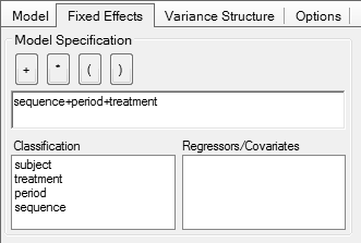
To obtain Type III result by \(\small{(3)}\), enter in the first field
sequence and in the second
subject(sequence). Note that you
cannot drag/drop them from the Classification.
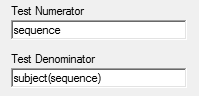
Note the additional row 6 giving the result and row 7 showing which effect is used as the denominator:
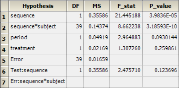
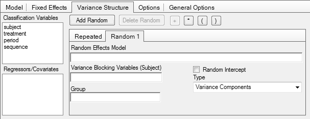
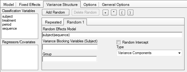
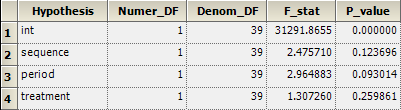
In the setup of a mixed-effects model in Phoenix WinNonlin, i.e., if subject(sequence) is specified as a random effect, the correct test is automatically performed:
In SAS
Test?
A statistical method to ‘adjust’ (i.e., correct) for a true sequence effect does not – and will never – exist. The bias due to unequal carryover can only be avoided by design.22
- The study is performed in healthy subjects or patients with a stable disease,
- the drug is not an endogenous entity, and
- an adequate washout is maintained (no pre-dose concentrations in higher periods).
Although guidelines mention only ‘no pre-dose concentrations in higher periods’ to confirm absence of carryover, this is just the most obvious part of the game. In order to get an unbiased estimate of the treatment effect, subjects have to be in the same physiological state in higher periods than in the drug-naïve first. Some drugs influence their own pharmacokinetics, i.e., are auto-inducers or -inhibitors.23
Say, the washout of a 2×2×2 crossover was planned based on the reported half life after a single dose in such a way that no pre-dose concentrations in the second period were expected.
- If the drug is an auto-inducer, concentrations in the second period will be lower than in the first.
- If the drug is an auto-inhibitor, concentrations in the second period will be higher than in the first.
In such cases, assessing the pre-dose concentrations is not sufficient. Possibly a significant period effect can be seen in the ANOVA. However, it is a misconceception that the period effect will cancel out as usual. If the true bioavailabilities are not exactly equal, the estimated treatment effect will be biased. It is necessary to prolong the washout in order to allow the metabolizing system to return to its original state.
The topic of a suitable washout from a PK perspective will be covered in another article.
Grizzle proposed in 1965 the so-called ‘Two-stage Analysis’.24
- An F-test for a significant sequence effect at α = 0.10.25
- If p(F) < 0.10, evaluation of the first period as a parallel design.
- Otherwise, evaluate the study as a crossover.
if (anova(model)["sequence", "Pr(>F)"] < 0.1) {
  mod.par <- lm(logPK ~ treatment,
                        data[data$period == 1, ])
}
To quote one of the pioneers of bioequivalence:
“Note that the carryover effect is, essentially, the sequence effect, which can be tested against the sum of squares within sequence. If this carryover effect exists, then it confounds the test on formulations. […] My own experience with a large number of comparative bioavailability trials has led me to believe that significant carryover effects (at the 0.05 level) tend to occur in about 5% of the trials; in other words, I believe that carryover effects do not normally exist.
In 1989 Freeman demonstrated that Grizzle’s ‘Two-stage Analysis’ is statistically flawed and should be avoided because it leads not only to biased estimates but – as any preliminary test – inflates the Type I Error.26
The FDA rightly stated about testing at \(\small{\alpha=0.1}\):
“Even if there were no true sequence effect, no unequal residual effects, and no period-by-treatment statistical interaction, approximately ten out of one hundred standard two-treatment crossover studies would be likely to show an apparent sequence effect, if the testing is carried out at the ten percent level of significance.
If the ANOVA test for the presence of a sequence effect result in statistical significance, the actual cause cannot be determine from the data alone.
This theoretical consideration was confirmed in a meta-study of well-controlled crossover trials (324 in a 2×2×2 crossover and 96 in a 3×6×3 Williams’ design).28 As expected, a significant sequence effect was observed at approximately the level of the test and hence, was considered a statistical artifact.
From the diary of a consultant.29
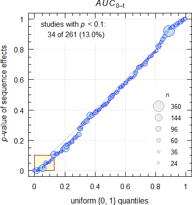
Fig. 1 Data from my archive.
I see more than the expected 10%… Likely I’m a victim of selection bias because regularly I get corpses on my desk to perform a – rarely useful – autopsy.30
Parts of Stephen Senn’s textbook31 can be understood as an essay against ‘adjusting’ for carryover. My personal interpretation is that – if conditions stated above hold – even testing for a sequence effect should be abandoned. In a later publication we find:
“Testing for carryover in bioequivalence studies […] is not recommended and, moreover, can be harmful. It seems that whenever carry-over is ‘detected’ under such conditions, it is a false positive and researchers will be led to use an inferior estimate, abandoning a superior one.
In the same sense:
“Our advice therefore is to avoid having a test for a carry-over difference by doing all that is possible to remove the possibility that such a difference will exist. This requires using wash-out periods of adequate length between the treatment periods.
According to the Consolidated Standards of Reporting Trials:34
“In particular, given that a carry over effect can neither be identified with sufficient power, nor can adjustment be made for such an effect in the 2×2 crossover design, the assumption needs to be made that any carry over effects are negligible and some justification presented for this. The description of the design should make clear how many interventions were tested, through how many periods, including information on the length of the treatment, run in, and washout periods (if any).
The EMA’s draft bioequivalence guideline stated:
“[…] tests for difference and the respective confidence intervals for the treatment effect, the period effect, and the sequence effect should be reported for descriptive assessment.
It’s laudable that the statement about tests and their reporting was removed in the final guideline:
“The statistical analysis should take into account sources of variation that can be reasonably assumed to have an effect on the response variable.
A test for carry-over is not considered relevant and no decisions regarding the analysis (e.g. analysis of the first period only) should be made on the basis of such a test. The potential for carry-over can be directly addressed by examination of the pre-treatment plasma concentrations in period 2 (and beyond if applicable).
Alas, Health Canada states in the current guidance:
“A summary of the testing of sequence, period and formulation effects should be presented. Explanations for significant effects should be given.
There is nothing to be ‘explained’. Oh dear, the period effect cancels out! For the lacking relevance of a significant formulation effect see another article.
Thank goodness, a test is not mentioned by the FDA in the latest draft guidance. Of course:
“An adequate washout period (e.g., more than five half-lives of the moieties to be measured) should separate each treatment.
We recommend that if the pre-dose value is > 5 percent of the Cmax, applicants drop the subject from all BE study evaluations.
Similar in the draft guideline of the ICH:
“A test for carry-over is not considered relevant and no decisions regarding the analysis, e.g., analysis of the first period only, should be made on the basis of such a test. In crossover studies, the potential for carry-over can be directly addressed by examination of the pre-treatment plasma concentrations in period 2 and beyond if applicable, e.g., period 3 in a 3-period study.
If there are subjects for whom the pre-dose concentration is greater than 5% of the Cmax value for the subject in that period, then the pivotal statistical analysis should be performed excluding the data from that subject.
Simulations
Here we face a situation where we need simulations. Except in a meta-study, retrospectively assessing a particular study is of no value, as we neither know if a true carryover was present and, if so, its extent.
Single study
The simulations are based on \(\small{\log_{e}}\) normal distributed data, true T/R-ratio 0.95, true CV 0.25, n 28 (balanced sequences), and a small period effect \(\small{\pi_2=+0.02}\) (responses in the second period are 2% higher than in the first).
Note how the sequence effect is tested. In the first example below we get an \(\small{F}\)-value of \(\small{0.0817/0.339\approx0.241}\) by \(\small{(3)}\) instead of \(\small{0.0817/0.0557\approx1.468}\) by \(\small{(2)}\). Only the former is correct \(\small{(p(F)\approx0.628}\) instead of \(\small{p(F)\approx0.237)}\).
As expected, we see a significant subject effect because \(\small{s_\textrm{b}^2>s_\textrm{w}^2}\) and subjects are different indeed. If you see in a particular study a subject effect which is not highly significant, that’s a suspicious case.
We need a supportive function for the simulations. Cave: 165 LOC.
sim.effects <- function(alpha = 0.05, theta0 = 0.95,
                        CV = 0.25, CVb, n = 28L,
                        per.effect = c(0, 0),
                        carryover = c(0, 0)) {
  if (length(per.effect) == 1) per.effect <- c(0, per.effect)
  # carryover: first element R -> T, second element T -> R
  set.seed(123456789)
  if (missing(CVb)) CVb <- CV * 1.5 # arbitrary
  sd     <- sqrt(log(CV^2 + 1))
  sd.b   <- sqrt(log(CVb^2 + 1))
  subj   <- 1:n
  # within subjects
  T      <- rnorm(n = n, mean = log(theta0), sd = sd)
  R      <- rnorm(n = n, mean = 0, sd = sd)
  # between subjects
  TR     <- rnorm(n = n, mean = 0, sd = sd.b)
  T      <- T + TR
  R      <- R + TR
  TR.sim <- exp(mean(T) - mean(R))
  data   <- data.frame(subject   = rep(subj, each = 2),
                       period    = 1:2L,
                       sequence  = c(rep("RT", n),
                                     rep("TR", n)),
                       treatment = c(rep(c("R", "T"), n/2),
                                     rep(c("T", "R"), n/2)),
                       logPK     = NA_real_)
  subj.T <- subj.R <- 0L    # subject counters
  for (i in 1:nrow(data)) {# clumsy but transparent
    if (data$treatment[i] == "T") {
      subj.T  <- subj.T + 1L
      if (data$period[i] == 1L) {
        data$logPK[i] <- T[subj.T] + per.effect[1]
      } else {
        data$logPK[i] <- T[subj.T] + per.effect[2] + carryover[1]
      }
    } else {
      subj.R  <- subj.R + 1L
      if (data$period[i] == 1L) {
        data$logPK[i] <- R[subj.R] + per.effect[1]
      } else {
        data$logPK[i] <- R[subj.T] + per.effect[2] + carryover[2]
      }
    }
  }
  per.mean  <- exp(c(mean(data$logPK[data$period == 1]),
                     mean(data$logPK[data$period == 2])))
  seq.mean  <- exp(c(mean(data$logPK[data$sequence == "RT"]),
                     mean(data$logPK[data$sequence == "TR"])))
  trt.mean  <- exp(c(mean(data$logPK[data$treatment == "R"]),
                     mean(data$logPK[data$treatment == "T"])))
  cs        <- c("subject", "period", "sequence", "treatment")
  data[cs]  <- lapply(data[cs], factor)
  typeIII.h <- c(paste("Type III ANOVA Table: Crossover"),
                       "sequence vs")
  model     <- lm(logPK ~ sequence + subject%in%sequence +
                          period + treatment, data = data)
  TR.est    <- exp(coef(model)[["treatmentT"]])
  CI        <- as.numeric(exp(confint(model, "treatmentT",
                                      level = 1 - 2 * alpha)))
  m.form    <- toString(model$call)
  m.form    <- substr(m.form, 5, nchar(m.form)-6)
  typeIII<- anova(model)
  attr(typeIII, "heading")[1] <- m.form
  if ("sequence:subject" %in% rownames(typeIII)) {# nested
    MSdenom <- typeIII["sequence:subject", "Mean Sq"]
    df2     <- typeIII["sequence:subject", "Df"]
  } else {                                        # simple
    MSdenom <- typeIII["subject", "Mean Sq"]
    df2     <- typeIII["subject", "Df"]
  }
  fvalue <- typeIII["sequence", "Mean Sq"] / MSdenom
  df1    <- typeIII["sequence", "Df"]
  typeIII["sequence", 4]      <- fvalue
  typeIII["sequence", 5]      <- pf(fvalue, df1, df2,
                                    lower.tail = FALSE)
  attr(typeIII, "heading")[2:3] <- typeIII.h[1]
  if ("sequence:subject" %in% rownames(typeIII)) {
    attr(typeIII, "heading")[3] <- paste(typeIII.h[2],
                                         "sequence:subject")
  } else {
    attr(typeIII, "heading")[3] <- paste(typeIII.h[2],
                                         "subject")
  }
  CV.est <- sqrt(exp(typeIII["Residuals", "Mean Sq"])-1)
  print(typeIII, digits = 4, signif.legend = FALSE)
  if (typeIII["sequence", "Pr(>F)"] < 0.1) {# ‘Two-stage analysis’
    mod.par    <- lm(logPK ~ treatment, data[data$period == 1, ])
    TR.par.est <- exp(coef(mod.par)[["treatmentT"]])
    CI.par     <- as.numeric(exp(confint(mod.par, "treatmentT",
                                         level = 1 - 2 * alpha)))
    aovPar     <- anova(mod.par)
    m.form     <- toString(mod.par$call)
    m.form     <- substr(m.form, 5, nchar(m.form)-26)
    attr(aovPar, "heading")[1] <- paste0("\n", m.form)
    attr(aovPar, "heading")[2] <- "ANOVA Table: Period 1 parallel"
    CV.par.est <- sqrt(exp(aovPar["Residuals", "Mean Sq"])-1)
    print(aovPar, digits = 4, signif.legend = FALSE)
  }
  txt <- paste("\ntheta0                  ",
               sprintf("%.4f", theta0),
               "\nPeriod effect    (1, 2)",
               paste(sprintf("%+g", per.effect), collapse = ", "),
               "\nCarryover  (R->T, T->R)",
               paste(sprintf("%+g", carryover), collapse = ", "),
               "\nPeriod means     (1, 2) ",
               paste(sprintf("%.4f", per.mean),
               collapse = ", "),
               "\nSequence means (RT, TR) ",
               paste(sprintf("%.4f", seq.mean),
               collapse = ", "),
               "\nTreatment means  (R, T) ",
               paste(sprintf("%.4f", trt.mean),
               collapse = ", "),
               "\nSimulated T/R-ratio     ",
               sprintf("%.4f", TR.sim))
  if (typeIII["sequence", "Pr(>F)"] < 0.1) {
    txt <- paste(txt, "\n\n    Analysis of both periods")
  } else {
    txt <- paste(txt, "\n")
  }
  txt <- paste(txt, "\nEstimated T/R-ratio     ",
               sprintf("%.4f", TR.est),
               "\nBias                   ")
  if (sqrt(.Machine$double.eps) >= abs(TR.est - TR.sim)) {
    txt <- paste(txt, "\u00B10.00%")
  } else {
    txt <- paste(txt, sprintf("%+.2f%%",
                 100*(TR.est-TR.sim)/TR.sim))
  }
  txt <- paste(txt, sprintf("%s%.f%% %s",
               "\n", 100*(1-2*alpha),
               "CI                  "),
               paste(sprintf("%.4f", CI),
               collapse = " \u2013 "))
  if (round(CI[1], 4) >= 0.80 &
      round(CI[2], 4) <= 1.25) {
    txt <- paste(txt, "(pass)")
  } else {
    txt <- paste(txt, "(fail)")
  }
  txt <- paste(txt, "\nEstimated CV (within)   ",
               sprintf("%.4f", CV.est))
  if (typeIII["sequence", "Pr(>F)"] < 0.1) {
    txt <- paste(txt, "\n\n    Analysis of first period",
                  "\nEstimated T/R-ratio     ",
                  sprintf("%.4f", TR.par.est),
                  "\nBias                   ",
                  sprintf("%+.2f%%",
                  100*(TR.par.est-TR.sim)/TR.sim),
                  paste0("\n",
                  sprintf("%.f%% CI                  ",
                  100*(1-2*alpha))),
                  paste(sprintf("%.4f", CI.par),
                  collapse = " \u2013 "))
    if (round(CI.par[1], 4) >= 0.80 &
        round(CI.par[2], 4) <= 1.25) {
      txt <- paste(txt, "(pass)")
    } else {
      txt <- paste(txt, "(fail)")
    }
    txt <- paste(txt, "\nEstimated CV (total)    ",
                 sprintf("%.4f", CV.par.est))
  }
  cat(txt, "\n")
}
ANOVA tables’ significance codes
. <0.1 & ≥0.05
* <0.05 & ≥0.01
** <0.01 & ≥0.001
*** <0.001Case 1
Small period effect, large but equal carryover; \(\small{\pi_2=+0.02,\,\lambda_\textrm{R}=\lambda_\textrm{T}=+0.2}\).
sim.effects(theta0 = 0.95, CV = 0.25, n = 28,
            per.effect = +0.02, carryover = c(+0.2, +0.2))
# logPK ~ sequence + subject %in% sequence + period + treatment
# Type III ANOVA Table: Crossover
# sequence vs sequence:subject
# Df Sum Sq Mean Sq F value Pr(>F)
# sequence 1 0.082 0.0817 0.241 0.627562
# period 1 0.875 0.8746 15.709 0.000514 ***
# treatment 1 0.031 0.0309 0.554 0.463251
# sequence:subject 26 8.814 0.3390 6.089 8.52e-06 ***
# Residuals 26 1.448 0.0557
#
# theta0 0.9500
# Period effect (1, 2) +0, +0.02
# Carryover (R->T, T->R) +0.2, +0.2
# Period means (1, 2) 1.0101, 1.2970
# Sequence means (RT, TR) 1.1017, 1.1892
# Treatment means (R, T) 1.1718, 1.1180
# Simulated T/R-ratio 0.9541
#
# Estimated T/R-ratio 0.9541
# Bias ±0.00%
# 90% CI 0.8568 – 1.0625 (pass)
# Estimated CV (within) 0.2393The sequence effect is not significant at the 0.1 level. Significant period effect, unbiased T/R-ratio. All is good, since the carryover cancels out.
Case 2
Small period effect, large but unequal carryover; \(\small{\pi_2=+0.02,\,\lambda_\textrm{R}=+0.05,\,\lambda_\textrm{T}=+0.2}\).
sim.effects(theta0 = 0.95, CV = 0.25, n = 28,
            per.effect = +0.02, carryover = c(+0.05, +0.20))
# logPK ~ sequence + subject %in% sequence + period + treatment
# Type III ANOVA Table: Crossover
# sequence vs sequence:subject
# Df Sum Sq Mean Sq F value Pr(>F)
# sequence 1 0.321 0.3209 0.947 0.3395
# period 1 0.428 0.4285 7.696 0.0101 *
# treatment 1 0.208 0.2082 3.740 0.0641 .
# sequence:subject 26 8.814 0.3390 6.089 8.52e-06 ***
# Residuals 26 1.448 0.0557
#
# theta0 0.9500
# Period effect (1, 2) +0, +0.02
# Carryover (R->T, T->R) +0.05, +0.2
# Period means (1, 2) 1.0101, 1.2032
# Sequence means (RT, TR) 1.0221, 1.1892
# Treatment means (R, T) 1.1718, 1.0372
# Simulated T/R-ratio 0.9541
#
# Estimated T/R-ratio 0.8852
# Bias -7.23%
# 90% CI 0.7949 – 0.9857 (fail)
# Estimated CV (within) 0.2393The sequence effect is not significant at the 0.1 level but we get a
negatively biased T/R-ratio. Splendid – the study fails
although T and R are equivalent.
Note that the period effect is still significant but to great extent
‘masked’ (0.0101 instead of 0.000514).
Case 3
Small period effect, extremely unequal carryover; \(\small{\pi_2=+0.02,\,\lambda_\textrm{R}=+0.05,\,\lambda_\textrm{T}=+0.45}\).
sim.effects(theta0 = 0.95, CV = 0.25, n = 28,
            per.effect = +0.02, carryover = c(+0.05, +0.45))
# logPK ~ sequence + subject %in% sequence + period + treatment
# Type III ANOVA Table: Crossover
# sequence vs sequence:subject
# Df Sum Sq Mean Sq F value Pr(>F)
# sequence 1 1.070 1.0696 3.155 0.087400 .
# period 1 1.260 1.2596 22.623 6.39e-05 ***
# treatment 1 0.854 0.8538 15.335 0.000582 ***
# sequence:subject 26 8.814 0.3390 6.089 8.52e-06 ***
# Residuals 26 1.448 0.0557
#
# logPK ~ treatment
# ANOVA Table: Period 1 parallel
# Df Sum Sq Mean Sq F value Pr(>F)
# treatment 1 0.006 0.00607 0.031 0.862
# Residuals 26 5.100 0.19615
#
# theta0 0.9500
# Period effect (1, 2) +0, +0.02
# Carryover (R->T, T->R) +0.05, +0.45
# Period means (1, 2) 1.0101, 1.3634
# Sequence means (RT, TR) 1.0221, 1.3475
# Treatment means (R, T) 1.3278, 1.0372
# Simulated T/R-ratio 0.9541
#
# Analysis of both periods
# Estimated T/R-ratio 0.7812
# Bias -18.13%
# 90% CI 0.7015 – 0.8699 (fail)
# Estimated CV (within) 0.2393
#
# Analysis of first period
# Estimated T/R-ratio 1.0299
# Bias +7.94%
# 90% CI 0.7741 – 1.3702 (fail)
# Estimated CV (total) 0.4655The sequence effect is significant at the 0.1 level and we get an
extremely negatively biased T/R-ratio.
Analysis of the first period as a parallel design gives a
positively biased T/R-ratio (even the direction of the
difference of T from R changes).
Case 4
Small period effect, unequal carryover (opposite direction); \(\small{\pi_2=+0.02,\,\lambda_\textrm{R}=+0.075,\,\lambda_\textrm{T}=-0.075}\).
sim.effects(theta0 = 0.95, CV = 0.25, n = 28,
            per.effect = +0.02, carryover = c(+0.075, -0.075))
# logPK ~ sequence + subject %in% sequence + period + treatment
# Type III ANOVA Table: Crossover
# sequence vs sequence:subject
# Df Sum Sq Mean Sq F value Pr(>F)
# sequence 1 0.000 0.0000 0.000 0.993
# period 1 0.035 0.0349 0.627 0.436
# treatment 1 0.011 0.0110 0.198 0.660
# sequence:subject 26 8.814 0.3390 6.089 8.52e-06 ***
# Residuals 26 1.448 0.0557
#
# theta0 0.9500
# Period effect (1, 2) +0, +0.02
# Carryover (R->T, T->R) +0.075, -0.075
# Period means (1, 2) 1.0101, 1.0619
# Sequence means (RT, TR) 1.0349, 1.0364
# Treatment means (R, T) 1.0212, 1.0503
# Simulated T/R-ratio 0.9541
#
# Estimated T/R-ratio 1.0284
# Bias +7.79%
# 90% CI 0.9236 – 1.1452 (pass)
# Estimated CV (within) 0.2393The sequence effect is not significant (actually close to 1)
but the T/R-ratio extremely positively biased.
The period effect is not significant any more (0.436 instead of
0.000514).
This example demonstrates the absurdity of testing a sequence effect. The ANOVA looks completely ‘normal’, none of the effects is significant. Study passes, everybody happy, questions from an assessor unlikely.
Nevertheless, the estimated T/R-ratio is outright wrong. One gets the
false impression that T ist slightly more bioavailable than R, whereas
the truth is the other way ’round. The true but unknown
carryovers ‘pulled’ the responses of T up and ‘pushed’ the ones of R
down.
Here we know it. In reality we don’t have a clue.
Multiple studies
We can also simulate a large number of studies. Results of a
simulation are provided in the res data.frame in full
numeric precision. Cave:
158 LOC.
If you want to simulate more than 50,000 studies, use the optional
argument progress = TRUE in the function call. One million
take on my machine a couple of hours to complete and the progress bar
gives an idea how many are already finished.
sim.study <- function(CV, CVb, theta0, targetpower,
                      per.effect = c(0, 0),
                      carryover = c(0, 0),
                      nsims, setseed = TRUE,
                      progress = FALSE, # TRUE for a progress bar
                      print = TRUE) {
  library(PowerTOST)
  if (missing(CV)) stop("CV must be given.")
  if (missing(CVb)) CVb <- CV * 1.5 # arbitrary
  if (missing(theta0)) stop("theta0 must be given.")
  if (length(per.effect) == 1) per.effect <- c(0, per.effect)
  if (missing(targetpower)) stop("targetpower must be given.")
  if (missing(nsims)) stop("nsims must be given.")
  if (setseed) set.seed(123456)
  tmp <- sampleN.TOST(CV = CV, theta0 = theta0,
                      targetpower = targetpower,
                      print = FALSE, details = FALSE)
  n    <- tmp[["Sample size"]]
  pwr  <- tmp[["Achieved power"]]
  res  <- data.frame(p = rep(NA_real_, nsims), PE = NA_real_,
                     Bias = NA_real_, lower = NA_real_,
                     upper = NA_real_, BE = FALSE, sig = FALSE)
  sd   <- CV2se(CV)
  sd.b <- CV2se(CVb)
  if (progress) pb <- txtProgressBar(0, 1, 0, char = "\u2588",
                                     width = NA, style = 3)
  for (sim in 1:nsims) {
    subj   <- 1:n
    T      <- rnorm(n = n, mean = log(theta0), sd = sd)
    R      <- rnorm(n = n, mean = 0, sd = sd)
    TR     <- rnorm(n = n, mean = 0, sd = sd.b)
    T      <- T + TR
    R      <- R + TR
    TR.sim <- exp(mean(T) - mean(R))
    data   <- data.frame(subject   = rep(subj, each = 2),
                         period    = 1:2L,
                         sequence  = c(rep("RT", n),
                                       rep("TR", n)),
                         treatment = c(rep(c("R", "T"), n/2),
                                       rep(c("T", "R"), n/2)),
                         logPK     = NA_real_)
    subj.T <- subj.R <- 0L
    for (i in 1:nrow(data)) {
      if (data$treatment[i] == "T") {
        subj.T  <- subj.T + 1L
        if (data$period[i] == 1L) {
          data$logPK[i] <- T[subj.T] + per.effect[1]
        } else {
          data$logPK[i] <- T[subj.T] + per.effect[2] + carryover[1]
        }
      } else {
        subj.R  <- subj.R + 1L
        if (data$period[i] == 1L) {
          data$logPK[i] <- R[subj.R] + per.effect[1]
        } else {
          data$logPK[i] <- R[subj.T] + per.effect[2] + carryover[2]
        }
      }
    }
    cs       <- c("subject", "period", "sequence", "treatment")
    data[cs] <- lapply(data[cs], factor)
    # simple model for speed reasons
    model    <- lm(logPK ~ sequence + subject + period +
                           treatment, data = data)
    PE       <- exp(coef(model)[["treatmentT"]])
    CI       <- exp(confint(model, "treatmentT",
                            level = 1 - 2 * 0.05))
    typeIII  <- anova(model)
    MSdenom  <- typeIII["subject", "Mean Sq"]
    df2      <- typeIII["subject", "Df"]
    fvalue   <- typeIII["sequence", "Mean Sq"] / MSdenom
    df1      <- typeIII["sequence", "Df"]
    typeIII["sequence", 4] <- fvalue
    typeIII["sequence", 5] <- pf(fvalue, df1, df2,
                                 lower.tail = FALSE)
    res[sim, 1:5] <- c(typeIII["sequence", 5], PE,
                     100 * (PE - theta0) / theta0, CI)
    if (round(CI[1], 4) >= 0.80 & round(CI[2], 4) <= 1.25)
      res[sim, 6] <- TRUE
    if (res$p[sim] < 0.1) res$sig[sim] <- TRUE
    if (progress) setTxtProgressBar(pb, sim/nsims)
  }
  if (print) {
    p   <- sum(res$BE) # passed
    f   <- nsims - p   # failed
    txt <- paste("Simulation scenario",
                 "\n  CV               :", sprintf("%7.4f", CV),
                 "\n  theta0           :", sprintf("%7.4f", theta0),
                 "\n  n                :", n,
                 "\n  achieved power   :", sprintf("%7.4f", pwr))
    if (sum(per.effect) == 0) {
      txt <- paste(txt, "\n  no period effects")
    } else {
      txt <- paste(txt, "\n  period effects   :",
                   sprintf("%+.3g,", per.effect[1]),
                   sprintf("%+.3g", per.effect[2]))
    }
    if (length(unique(carryover)) == 1) {
      if (sum(carryover) == 0) {
        txt <- paste0(txt, ", no carryover")
      } else {
        txt <- paste(txt, "\n  equal carryover  :",
                     sprintf("%+.3g", unique(carryover)))
      }
    } else {
      txt <- paste(txt, "\n  unequal carryover:",
                   sprintf("%+.3g,", carryover[1]),
                   sprintf("%+.3g", carryover[2]))
    }
    txt <- paste(txt,
                 paste0("\n", formatC(nsims, big.mark = ",")),
                 "simulated studies",
                 "\n  Significant sequence effect:",
                  sprintf("%6.2f%%", 100 * sum(res$sig) / nsims),
                  "\n  PE   (median, quartiles)   :",
                  sprintf("%8.4f", median(res$PE)),
                  sprintf("(%.4f, %.4f)",
                  quantile(res$PE, probs = 0.25),
                  quantile(res$PE, probs = 0.75)),
                  "\n  Bias (median, quartiles)   :",
                  sprintf("%+6.2f%%", median(res$Bias)),
                  sprintf("(%+.2f%%, %+.2f%%)",
                  quantile(res$Bias, probs = 0.25),
                  quantile(res$Bias, probs = 0.75)),
                  paste0("\n", formatC(p, big.mark = ",")), "passing studies",
                  sprintf("(empiric power %.4f)", p / nsims),
                  "\n  Significant sequence effect:",
                  sprintf("%6.2f%%", 100 * sum(res$sig[res$BE == TRUE]) / p),
                  "\n  PE   (median, quartiles)   :",
                  sprintf("%8.4f", median(res$PE[res$BE == TRUE])),
                  sprintf("(%.4f, %.4f)",
                  quantile(res$PE[res$BE == TRUE], probs = 0.25),
                  quantile(res$PE[res$BE == TRUE], probs = 0.75)),
                  "\n  Bias (median, quartiles)   :",
                  sprintf("%+6.2f%%", median(res$Bias[res$BE == TRUE])),
                  sprintf("(%+.2f%%, %+.2f%%)",
                  quantile(res$Bias[res$BE == TRUE], probs = 0.25),
                  quantile(res$Bias[res$BE == TRUE], probs = 0.75)),
                  paste0("\n", formatC(f, big.mark = ",")), "failed studies",
                  sprintf("(empiric type II error %.4f)", f / nsims),
                  "\n  Significant sequence effect:",
                  sprintf("%6.2f%%", 100 * sum(res$sig[res$BE == FALSE]) / f),
                  "\n  PE   (median, quartiles)   :",
                  sprintf("%8.4f", median(res$PE[res$BE == FALSE])),
                  sprintf("(%.4f, %.4f)",
                  quantile(res$PE[res$BE == FALSE], probs = 0.25),
                  quantile(res$PE[res$BE == FALSE], probs = 0.75)),
                  "\n  Bias (median, quartiles)   :",
                  sprintf("%+6.2f%%", median(res$Bias[res$BE == FALSE])),
                  sprintf("(%+.2f%%, %+.2f%%)",
                  quantile(res$Bias[res$BE == FALSE], probs = 0.25),
                  quantile(res$Bias[res$BE == FALSE], probs = 0.75)), "\n")
    cat(txt)
  }
  if (progress) close(pb)
  return(res)
  rm(res)
}
Scenario 1
No period effect, no carryover (first condition from above); \(\small{\pi_1=\pi_2=0,\,\lambda_\textrm{R}=\lambda_\textrm{T}=0}\).
res <- sim.study(CV = 0.25, theta0 = 0.94,
                 targetpower = 0.80, nsims = 5e4L)
# Simulation scenario
# CV : 0.2500
# theta0 : 0.9400
# n : 32
# achieved power : 0.8180
# no period effects, no carryover
# 50,000 simulated studies
# Significant sequence effect: 10.09%
# PE (median, quartiles) : 0.9396 (0.9021, 0.9796)
# Bias (median, quartiles) : -0.04% (-4.04%, +4.21%)
# 40,989 passing studies (empiric power 0.8198)
# Significant sequence effect: 10.05%
# PE (median, quartiles) : 0.9528 (0.9230, 0.9884)
# Bias (median, quartiles) : +1.36% (-1.80%, +5.15%)
# 9,011 failed studies (empiric type II error 0.1802)
# Significant sequence effect: 10.31%
# PE (median, quartiles) : 0.8658 (0.8464, 0.8800)
# Bias (median, quartiles) : -7.90% (-9.96%, -6.38%)As expected: Although there is no true sequence effect, we detect a significant one at approximately the level of test. Hence, we fell into the trap of false positives.
Scenario 2
No period effect and large positive – equal – carryover (first condition from above); \(\small{\pi_1=\pi_2=0,\,\lambda_\textrm{R}=\lambda_\textrm{T}=+0.1}\).
res <- sim.study(CV = 0.25, theta0 = 0.94,
                 targetpower = 0.80, nsims = 5e4L,
                 carryover = c(+0.1, +0.1))
# Simulation scenario
# CV : 0.2500
# theta0 : 0.9400
# n : 32
# achieved power : 0.8180
# no period effects
# equal carryover : +0.1
# 50,000 simulated studies
# Significant sequence effect: 10.09%
# PE (median, quartiles) : 0.9396 (0.9021, 0.9796)
# Bias (median, quartiles) : -0.04% (-4.04%, +4.21%)
# 40,989 passing studies (empiric power 0.8198)
# Significant sequence effect: 10.05%
# PE (median, quartiles) : 0.9528 (0.9230, 0.9884)
# Bias (median, quartiles) : +1.36% (-1.80%, +5.15%)
# 9,011 failed studies (empiric type II error 0.1802)
# Significant sequence effect: 10.31%
# PE (median, quartiles) : 0.8658 (0.8464, 0.8800)
# Bias (median, quartiles) : -7.90% (-9.96%, -6.38%)As expected identical to Scenario 1 simulated without carryover.
Scenario 3
A small positive period effect and small unequal carryover with opposite direction (third condition from above); \(\small{\pi_1=0,\,\pi_2=+0.02,\,\lambda_\textrm{R}=+0.02,\,\lambda_\textrm{T}=-0.02}\).
res <- sim.study(CV = 0.25, theta0 = 0.94,
                 targetpower = 0.80, nsims = 5e4L,
                 per.effect = 0.02, carryover = c(+0.02, -0.02))
# Simulation scenario
# CV : 0.2500
# theta0 : 0.9400
# n : 32
# achieved power : 0.8180
# period effects : +0, +0.02
# unequal carryover: +0.02, -0.02
# 50,000 simulated studies
# Significant sequence effect: 10.42%
# PE (median, quartiles) : 0.9586 (0.9203, 0.9994)
# Bias (median, quartiles) : +1.98% (-2.10%, +6.32%)
# 44,326 passing studies (empiric power 0.8865)
# Significant sequence effect: 10.39%
# PE (median, quartiles) : 0.9661 (0.9336, 1.0042)
# Bias (median, quartiles) : +2.78% (-0.68%, +6.83%)
# 5,674 failed studies (empiric type II error 0.1135)
# Significant sequence effect: 10.72%
# PE (median, quartiles) : 0.8700 (0.8524, 0.8846)
# Bias (median, quartiles) : -7.45% (-9.32%, -5.90%)Although there is a true unequal carryover, the percentage of studies where it is detected is not substantially above the false positive rate. Due to the unequal carryover on the average the Test treatment is ‘pushed up’ in the second period and the Reference treatment ‘pulled down’. Therefore, the bias is larger than in Scenario 2. Since we simulated a T/R-ratio < 1, the positive bias translates into higher power.
Scenario 4
No period effect and large unequal carryover with opposite direction (third condition from above); \(\small{\pi_1=\pi_2=0,\,\lambda_\textrm{R}=+0.09,\,\lambda_\textrm{T}=-0.11}\).
res <- sim.study(CV = 0.25, theta0 = 0.94,
                 targetpower = 0.80, nsims = 5e4L,
                 carryover = c(+0.09, -0.11))
# Simulation scenario
# CV : 0.2500
# theta0 : 0.9400
# n : 32
# achieved power : 0.8180
# no period effects
# unequal carryover: +0.09, -0.11
# 50,000 simulated studies
# Significant sequence effect: 17.89%
# PE (median, quartiles) : 1.0384 (0.9969, 1.0826)
# Bias (median, quartiles) : +10.47% (+6.06%, +15.17%)
# 44,845 passing studies (empiric power 0.8969)
# Significant sequence effect: 17.92%
# PE (median, quartiles) : 1.0313 (0.9930, 1.0688)
# Bias (median, quartiles) : +9.71% (+5.64%, +13.70%)
# 5,155 failed studies (empiric type II error 0.1031)
# Significant sequence effect: 17.69%
# PE (median, quartiles) : 1.1486 (1.1291, 1.1715)
# Bias (median, quartiles) : +22.19% (+20.11%, +24.62%)Here it gets really interesting. Carryover is detected above the false positive rate. Nice at a first look but in the vast majority of cases it will not be detected. Again, power is larger than expected and now the bias is massive. Although we simulated a T/R-ratio of 0.94, the median of passing studies is 1.0313 – right on the other side of the pond… Of course, we gain power.
Simulation Summary
Single studies
Recall that the simulated T/R-ratio, CV, n, and the period effect were identical in all cases, as was the resulting T/R-ratio with 0.9541 and the CV with 0.2393.
\[\small{\begin{array}{clccrcc} \text{Case} & True\;\text{carryover} & p(F) & \text{PE} & \text{Bias (%)} & \text{90% CI} & \text{BE}\\ \hline 1 & \lambda_\textrm{R}=\lambda_\textrm{T}=+0.20 & 0.6276 & 0.9541 & \pm 0.00 & 0.8568-1.0625 & \text{pass}\\ 2 & \lambda_\textrm{R}=+0.050,\,\lambda_\textrm{T}=+0.20 & 0.3395 & 0.8852 & {\color{Red}{-7.23}} & 0.7949-0.9857 & \text{fail}\\ 3 & \lambda_\textrm{R}=+0.060,\,\lambda_\textrm{T}=+0.45 & {\color{Red}{0.0874}} & 0.7812 & {\color{Red}{-18.12}} & 0.7015-0.8699 & \text{fail}\\ 4 & \lambda_\textrm{R}=+0.075,\,\lambda_\textrm{T}=-0.75 & 0.9930 & 1.0284 & {\color{Red}{+7.79}} & 0.9236-1.1452 & \text{pass}\\ \hline\end{array}}\] Only if carryover is identical (Case 1) we get an unbiased estimate. Note that only in Case 3 a sequence effect is ‘detected’. In Case 4 with extremely different carryover the study passes but the point estimate gives a false impression (\(\small{f_\textrm{T}>f_\textrm{R}}\)).
Interlude 2For an assumed T/R-ratio 0.94 and CV 0.25 studies were powered with ≥0.80 (n 32 achieves 0.818). How to estimate the sample size is shown in another article. No period effect.
sim.effects(theta0 = 0.94, CV = 0.25, n = 32)
sim.effects(theta0 = 0.94, CV = 0.25, n = 32,
            carryover = c(+0.001, -0.001))
The 1st study (\(\small{\lambda_\textrm{R}=\lambda_\textrm{T}=0,\,p(F)\sim0.452}\))
fails.41
The 2nd with extremly small but unequal carryover (\(\small{\lambda_\textrm{R}=+0.001,\,\lambda_\textrm{T}=-0.001,\,p(F)\sim0.457}\))
passes.
A question to my regulatory friends: Disturbing, isn’t it?
Well roared, lion! Strictly speaking this is only correct if sequences are balanced.
For an assumed T/R-ratio 0.94 and CV 0.25 studies were powered with ≥0.80 (n 32 achieves 0.818). No carry-over but a massive period effect \(\small{\pi_2=0.2}\), i.e., 20% higher responses in the second period.
res <- sim.study(CV = 0.25, theta0 = 0.94,
                 targetpower = 0.80, nsims = 5e4L,
                 per.effect = 0.2)
# Simulation scenario
# CV : 0.2500
# theta0 : 0.9400
# n : 32
# achieved power : 0.8180
# period effects : +0, +0.2, no carryover
# 50,000 simulated studies
# Significant sequence effect: 10.09%
# PE (median, quartiles) : 0.9396 (0.9021, 0.9796)
# Bias (median, quartiles) : -0.04% (-4.04%, +4.21%)
# 40,989 passing studies (empiric power 0.8198)
# Significant sequence effect: 10.05%
# PE (median, quartiles) : 0.9528 (0.9230, 0.9884)
# Bias (median, quartiles) : +1.36% (-1.80%, +5.15%)
# 9,011 failed studies (empiric type II error 0.1802)
# Significant sequence effect: 10.31%
# PE (median, quartiles) : 0.8658 (0.8464, 0.8800)
# Bias (median, quartiles) : -7.90% (-9.96%, -6.38%)All is good. Note that this outcome is identical to Scenarios 1 and 2 above. That’s what we would expected.
However, if sequences get increasingly imbalanced, there might be a problem. Conditions like above but extreme imbalance.
sim.imb <- function(CV, CVb, theta0, targetpower,
                    per.effect = c(0, 0),
                    carryover = c(0, 0),
                    nsims, setseed = TRUE,
                    progress = FALSE, # TRUE for a progress bar
                    print = TRUE) {
  library(PowerTOST)
  if (missing(CV)) stop("CV must be given.")
  if (missing(CVb)) CVb <- CV * 1.5 # arbitrary
  if (missing(theta0)) stop("theta0 must be given.")
  if (length(per.effect) == 1) per.effect <- c(0, per.effect)
  if (missing(targetpower)) stop("targetpower must be given.")
  if (missing(nsims)) stop("nsims must be given.")
  if (setseed) set.seed(123456)
  tmp <- sampleN.TOST(CV = CV, theta0 = theta0,
                      targetpower = targetpower,
                      print = FALSE, details = FALSE)
  n    <- tmp[["Sample size"]]
  pwr  <- tmp[["Achieved power"]]
  res  <- data.frame(p = rep(NA_real_, nsims), PE = NA_real_,
                     Bias = NA_real_, lower = NA_real_,
                     upper = NA_real_, BE = FALSE, sig = FALSE)
  sd   <- CV2se(CV)
  sd.b <- CV2se(CVb)
  if (progress) pb <- txtProgressBar(0, 1, 0, char = "\u2588",
                                     width = NA, style = 3)
  for (sim in 1:nsims) {
    subj   <- 1:n
    T      <- rnorm(n = n, mean = log(theta0), sd = sd)
    R      <- rnorm(n = n, mean = 0, sd = sd)
    TR     <- rnorm(n = n, mean = 0, sd = sd.b)
    T      <- T + TR
    R      <- R + TR
    TR.sim <- exp(mean(T) - mean(R))
    data   <- data.frame(subject   = rep(subj, each = 2),
                         period    = 1:2L,
                         sequence  = c(rep("RT", n),
                                       rep("TR", n)),
                         treatment = c(rep(c("R", "T"), n/2),
                                       rep(c("T", "R"), n/2)),
                         logPK     = NA_real_)
    subj.T <- subj.R <- 0L
    for (i in 1:nrow(data)) {
      if (data$treatment[i] == "T") {
        subj.T  <- subj.T + 1L
        if (data$period[i] == 1L) {
          data$logPK[i] <- T[subj.T] + per.effect[1]
      }else {
          data$logPK[i] <- T[subj.T] + per.effect[2] + carryover[1]
        }
    }else {
        subj.R  <- subj.R + 1L
        if (data$period[i] == 1L) {
          data$logPK[i] <- R[subj.R] + per.effect[1]
      }else {
          data$logPK[i] <- R[subj.T] + per.effect[2] + carryover[2]
        }
      }
    }
    subj.TR  <- unique(data$subject[data$sequence == "TR"])
    remove   <- tail(subj.TR, ceiling(n / 3)) # sequences extremely imbalanced
    data     <- data[!data$subject %in% remove, ]
    cs       <- c("subject", "period", "sequence", "treatment")
    data[cs] <- lapply(data[cs], factor)
    # simple model for speed reasons
    model    <- lm(logPK ~ sequence + subject + period +
                           treatment, data = data)
    PE       <- exp(coef(model)[["treatmentT"]])
    CI       <- exp(confint(model, "treatmentT",
                            level = 1 - 2 * 0.05))
    typeIII  <- anova(model)
    MSdenom  <- typeIII["subject", "Mean Sq"]
    df2      <- typeIII["subject", "Df"]
    fvalue   <- typeIII["sequence", "Mean Sq"] / MSdenom
    df1      <- typeIII["sequence", "Df"]
    typeIII["sequence", 4] <- fvalue
    typeIII["sequence", 5] <- pf(fvalue, df1, df2,
                                 lower.tail = FALSE)
    res[sim, 1:5] <- c(typeIII["sequence", 5], PE,
                     100 * (PE - theta0) / theta0, CI)
    if (round(CI[1], 4) >= 0.80 & round(CI[2], 4) <= 1.25)
      res[sim, 6] <- TRUE
    if (res$p[sim] < 0.1) res$sig[sim] <- TRUE
    if (progress) setTxtProgressBar(pb, sim/nsims)
  }
  if (print) {
    p   <- sum(res$BE) # passed
    f   <- nsims - p   # failed
    txt <- paste("Simulation scenario",
                 "\n  CV               :", sprintf("%7.4f", CV),
                 "\n  theta0           :", sprintf("%7.4f", theta0),
                 "\n  n                :", n,
                 "\n  achieved power   :", sprintf("%7.4f", pwr))
    if (sum(per.effect) == 0) {
      txt <- paste(txt, "\n  no period effects")
  }else {
      txt <- paste(txt, "\n  period effects   :",
                   sprintf("%+.3g,", per.effect[1]),
                   sprintf("%+.3g", per.effect[2]))
    }
    if (length(unique(carryover)) == 1) {
      if (sum(carryover) == 0) {
        txt <- paste0(txt, ", no carryover")
    }else {
        txt <- paste(txt, "\n  equal carryover  :",
                     sprintf("%+.3g", unique(carryover)))
      }
  }else {
      txt <- paste(txt, "\n  unequal carryover:",
                   sprintf("%+.3g,", carryover[1]),
                   sprintf("%+.3g", carryover[2]))
    }
    txt <- paste(txt,
                 paste0("\n", formatC(nsims, big.mark = ",")),
                 "simulated studies",
                 "\n  Subjects in sequence RT    :",
                 length(unique(data$subject[data$sequence == "RT"])),
                 "\n  Subjects in sequence TR    :",
                 length(unique(data$subject[data$sequence == "TR"])),
                 "\n  Significant sequence effect:",
                  sprintf("%6.2f%%", 100 * sum(res$sig) / nsims),
                  "\n  PE   (median, quartiles)   :",
                  sprintf("%8.4f", median(res$PE)),
                  sprintf("(%.4f, %.4f)",
                  quantile(res$PE, probs = 0.25),
                  quantile(res$PE, probs = 0.75)),
                  "\n  Bias (median, quartiles)   :",
                  sprintf("%+6.2f%%", median(res$Bias)),
                  sprintf("(%+.2f%%, %+.2f%%)",
                  quantile(res$Bias, probs = 0.25),
                  quantile(res$Bias, probs = 0.75)),
                  paste0("\n", formatC(p, big.mark = ",")), "passing studies",
                  sprintf("(empiric power %.4f)", p / nsims),
                  "\n  Significant sequence effect:",
                  sprintf("%6.2f%%", 100 * sum(res$sig[res$BE == TRUE]) / p),
                  "\n  PE   (median, quartiles)   :",
                  sprintf("%8.4f", median(res$PE[res$BE == TRUE])),
                  sprintf("(%.4f, %.4f)",
                  quantile(res$PE[res$BE == TRUE], probs = 0.25),
                  quantile(res$PE[res$BE == TRUE], probs = 0.75)),
                  "\n  Bias (median, quartiles)   :",
                  sprintf("%+6.2f%%", median(res$Bias[res$BE == TRUE])),
                  sprintf("(%+.2f%%, %+.2f%%)",
                  quantile(res$Bias[res$BE == TRUE], probs = 0.25),
                  quantile(res$Bias[res$BE == TRUE], probs = 0.75)),
                  paste0("\n", formatC(f, big.mark = ",")), "failed studies",
                  sprintf("(empiric type II error %.4f)", f / nsims),
                  "\n  Significant sequence effect:",
                  sprintf("%6.2f%%", 100 * sum(res$sig[res$BE == FALSE]) / f),
                  "\n  PE   (median, quartiles)   :",
                  sprintf("%8.4f", median(res$PE[res$BE == FALSE])),
                  sprintf("(%.4f, %.4f)",
                  quantile(res$PE[res$BE == FALSE], probs = 0.25),
                  quantile(res$PE[res$BE == FALSE], probs = 0.75)),
                  "\n  Bias (median, quartiles)   :",
                  sprintf("%+6.2f%%", median(res$Bias[res$BE == FALSE])),
                  sprintf("(%+.2f%%, %+.2f%%)",
                  quantile(res$Bias[res$BE == FALSE], probs = 0.25),
                  quantile(res$Bias[res$BE == FALSE], probs = 0.75)), "\n")
    cat(txt)
  }
  if (progress) close(pb)
  return(res)
  rm(res)
}
res <- sim.imb(CV = 0.25, theta0 = 0.94,
targetpower = 0.80, per.effect = 0.2,
nsims = 5e4L)# Simulation scenario
# CV : 0.2500
# theta0 : 0.9400
# n : 32
# achieved power : 0.8180
# period effects : +0, +0.2, no carryover
# 50,000 simulated studies
# Subjects in sequence RT : 16
# Subjects in sequence TR : 5
# Significant sequence effect: 9.93%
# PE (median, quartiles) : 0.9395 (0.8851, 0.9977)
# Bias (median, quartiles) : -0.05% (-5.84%, +6.14%)
# 23,191 passing studies (empiric power 0.4638)
# Significant sequence effect: 10.34%
# PE (median, quartiles) : 0.9830 (0.9542, 1.0157)
# Bias (median, quartiles) : +4.57% (+1.52%, +8.05%)
# 26,809 failed studies (empiric type II error 0.5362)
# Significant sequence effect: 9.58%
# PE (median, quartiles) : 0.8897 (0.8513, 0.9249)
# Bias (median, quartiles) : -5.35% (-9.44%, -1.61%)We see that extreme imbalance together with a period effect will negatively affect power. Sure, because instead of 32 subjects we have only 21 eligible ones. That’s what we would expect:
power.TOST(CV = 0.25, theta0 = 0.94, n = c(16, 5))# [1] 0.4634564The estimate in passing studies will be biased as well.
Multiple studies
Recall that the simulated T/R-ratio, CV, and n were identical in all scenarios.
Results for all studies: \[\small{\begin{array}{clcrcr} \text{Scen.} & True\;\text{values} & \text{sim’s} & \text{sign. (%)} & \text{PE} & \text{Bias (%)}\\ \hline 1 &\small{\pi_2=\pm 0.00,\,\lambda_\textrm{R}=\lambda_\textrm{T}=\pm 0} & \text{50,000} & 10.09 & 0.9396 & -0.04\\ & & 10^6 & 9.95 & 0.9400 & \pm\text{0.00}\\ 2 & \small{\pi_2=+0.02,\,\lambda_\textrm{R}=\lambda_\textrm{T}=+0.1} & \text{50,000} & 10.09 & 0.9396 & -0.04\\ & & 10^6 & 9.95 & 0.9400 & \pm\text{0.00}\\ 3 & \small{\pi_2=+0.02,\,\lambda_\textrm{R}=+0.02,\,\lambda_\textrm{T}=-0.02} & \text{50,000} & 10.42 & 0.9586 & +1.98\\ & & 10^6 & 10.29 & 0.9590 & +2.02\\ 4 & \small{\pi_2=\pm 0.00,\,\lambda_\textrm{R}=+0.09,\,\lambda_\textrm{T}=-0.11} & \text{50,000} & 17.89 & 1.0384 & +10.47\\ & & 10^6 & 17.92 & 1.0316 & +9.74\\ \hline\end{array}}\] The slight bias in Scenarios 1 and 2 in 50,000 simulations is a negligible simulation artifact. It disappears in a larger number of simulations, as shown in one million simulations – demonstrating that the simulations are reliable. As expected, unequal carryover leads to biased estimates.
Results for the passing studies only (50,000 simulations): \[\small{\begin{array}{clrcrc}
\text{Scen.} & True\;\text{values} & \text{sign. (%)} &
\text{PE} & \text{Bias (%)} & \text{power}\\
\hline
1 &\small{\pi_2=\pm 0.00,\,\lambda_\textrm{R}=\lambda_\textrm{T}=\pm
0} & 10.05 & 0.9528 & +1.36 & 0.8198\\
2 & \small{\pi_2=+0.02,\,\lambda_\textrm{R}=\lambda_\textrm{T}=+0.1}
& 10.05 & 0.9528 & +1.36 & 0.8198\\
3 &
\small{\pi_2=+0.02,\,\lambda_\textrm{R}=+0.02,\,\lambda_\textrm{T}=-0.02}
& 10.39 & 0.9661 & +2.78 & 0.8865\\
4 & \small{\pi_2=\pm
0.00,\,\lambda_\textrm{R}=+0.09,\,\lambda_\textrm{T}=-0.11} & 17.92
& 1.0313 & +9.71 & 0.8969\\
\hline\end{array}}\] If there is no carryover (Scenario 1) or it
is equal (Scenario 2), the estimate is slightly biased because we
selected the passing studies only. The ∼10% of significant sequence
effects reflects the false positive rate.
The unequal carryover in Scenario 3 likely will not be detected (close
to the level of the test). Note that the bias is larger than in
Scenarios 1 and 2.
Scenario 4 is disturbing indeed. In ∼82% of studies the unequal
carryover of opposite direction will not be ‘detected’. The point
estimate gives a false impression (\(\small{f_\textrm{T}>f_\textrm{R}}\)).
There is a higher chance that studies will pass
BE (the empiric power is with ∼0.90
larger than the expected ∼0.82).
Any unequal carryover affects also the Type I Error (patient’s risk) if \(\small{f_\textrm{T}\leq f_\textrm{R}\,\wedge\,\lambda_\textrm{R}>\lambda_\textrm{T}}\) or \(\small{f_\textrm{T}\geq f_\textrm{R}\,\wedge\,\lambda_\textrm{R}<\lambda_\textrm{T}}\) because the estimate will be biased towards a ‘better’ value (i.e., closer to 1). That clearly demonstrates the importance of avoiding carryover by design.
Conclusion
“The combination of some data and an aching desire for an answer does not ensure that a reasonable answer can be extracted from a given body of data. “You can’t fix by analysis what you bungled by design. “[The] impatience with ambiguity can be criticized in the phrase:
Absence of evidence is not evidence of absence.
Apart from the theoretical considerations and Freeman’s proof26 given already 35 (‼) years ago, the simulations show that – even if the sequence effect is
not significant – in the case of a true unequal carryover the
estimated T/R-ratio will always be biased.
Due to the aliased effects, carryover cannot be estimated from the data
and hence, an ‘adjustment’ is not possible. Testing for a sequence
effect (unequal carryover) should be abandoned and a potential carryover
must be avoided by design.
On the other hand – as in any statistical test – a significant sequence effect may be pure chance, i.e., it does not prove that a true unequal carryover exists and thus, can be a false positive.
Coming back to the questions asked in the introduction. To repeat:
What is a significant sequence (carryover) effect … ?
It is a natural property of any test at level \(\small{\alpha}\) that it will be
significant even if the underlying condition (here a true
unequal carryover) does not exist.
Furthermore, in a nonreplicative design too many effects are aliased in
order to obtain an unequivocal answer.
… and do we have to care about one?
Not in particular. However, before you submit the study to an agency, assert that the correct test \(\small{(3)}\) was performed. Some CROs are notorious for applying the wrong one \(\small{(2)}\). Though the \(\small{p}\)-values of all effects are part of the software’s standard output, avoid a ‘proud’ verbatim statement in the report like »the sequence effect was not significant« (unless you apply to Health Canada). If \(\small{p<0.1}\), explain that it might be a false positive and point towards the – hopefully – appropriate design with sufficiently long washout period(s).
If the study was properly planned and only a limited number of pre-dose concentrations in higher periods were measured,45 there is nothing to worry about. If the number of excluded subjects is large, at least you learned to design the next study better.
Hoping that assessing the sequence effect can give viable information whether a study was properly designed and/or performed is simply futile.
If you are asked by a regulatory assessor for a ‘justification’, keep calm and answer in a diplomatic way.
If all information of a study is available (nature and
PK of the drug, in case of a drug
with nonlinear PK the dose, the
length of washout(s), the limit of quantification of the bioanalytical
method, eventual pre-dose concentrations), the study should be evaluated
as a crossover without testing the sequence effect.
However, if this is not the case (say for the reviewer of a journal), a
proposal could be considered.46
Open Question
What to do if we have to deal with an endogenous compound?
- Carryover considered »not unlikely« by the FDA.
- The EMA states:
»In bioequivalence studies with endogenous substances, it cannot be directly assessed whether carryover has occurred, so extra care should be taken to ensure that the washout period is of an adequate duration.«
I see. However, I fail to understand why baseline-corrected pre-dose concentrations \(\small{\mathsf{\tfrac{could}{should}}}\) not be used like the ones of other drugs. Is that meant by ‘indirectly assessed’?
A special case are biosimilars, where a true carryover is common. Hence, such studies should be performed in a parallel design.
Acknowledgment
Ana Henry, Simon Davis (Certara), Michael Tomashevskiy (OnTarget Group), and Martin Wolfsegger (Takeda) for helpful comments.
Licenses
 Helmut Schütz 2024
R and all packages GPL 3.0,
klippy MIT,
pandoc GPL 2.0.
1st version March 19, 2021. Rendered April 2, 2024 11:35 CEST
by rmarkdown
via pandoc in 0.54 seconds.
Footnotes and References
Labes D, Schütz H, Lang B. PowerTOST: Power and Sample Size for (Bio)Equivalence Studies. Package version 1.5.6. 2024-03-18. CRAN.↩︎
Pinheiro J, Bates D, DebRoy S, Sarkar D, EISPACK authors, Heisterkamp S, Van Willigen B, Ranke J, R-core. nlme: Linear and Nonlinear Mixed Effects Models. Package version 3.1.164. 2023-11-27. CRAN.↩︎
Bates D, Maechler M, Bolker B, Walker S, Haubo Bojesen Christensen R, Singmann H, Dai B, Scheipl F, Grothendieck G, Green P, Fox J, Bauer A, Krivitsky PN. lme4: Linear Mixed-Effects Models using ‘Eigen’ and S4. Package version 1.1.35.2. 2024-03-28. CRAN.↩︎
Kuznetsova A, Brockhoff PB, Haubo Bojesen Christensen R, Pødenphant Jensen S. lmerTest: Tests in Linear Mixed Effects Models. Package version 3.1.3. 2020-10-23. CRAN.↩︎
Statisticians may be more familiar with the terminology AB|BA.
Forgive me – in bioequivalence RT|TR is commonly used, where R denotes the Reference and T the Test treatment (formulation).↩︎Fleiss JL. The Design and Analysis of Clinical Experiments. New York: Wiley; 1986. p. 263.↩︎
Hauschke D, Steinijans V, Pigeot I. Bioequivalence Studies in Drug Development. Methods and Applications. Chichester: Wiley; 2007. ISBN 9780470094754.↩︎
No monozygotic twins or triplets in the study, if you don’t mind.↩︎
EMA, CHMP. Guideline on the Investigation of Bioequivalence. Subject accountability. London. 20 January 2010. Online. p 14.↩︎
Westlake WJ. Design and Evaluation of Bioequivalence Studies in Man. In: Blanchard J, Sawchuk RJ, Brodie BB, editors. Principles and perspectives in Drug Bioavailability. Basel: Karger; 1979. p. 192–210.↩︎
Westlake WJ. Bioavailability and Bioequivalence of Pharmaceutical Formulations. In: Peace KE, editor. Biopharmaceutical Statistics for Drug Development. New York: Marcel Dekker; 1988. p. 336–7.↩︎
Health Canada. Guidance Document: Conduct and Analysis of Comparative Bioavailability Studies. Ottawa. 2018/06/08. Online. p. 19.↩︎
Satterthwaite FE. An Approximate Distribution of Estimates of Variance Components. Biometrics Bulletin. 1946; 2(6): 110–4. doi:10.2307/3002019.↩︎
Kenward MG, Roger JH. Small Sample Inference for Fixed Effects from Restricted Maximum Likelihood. Biometrics. 1997; 53(3): 983–97. doi:10.2307/2533558.↩︎
Dallal GE. The Little Handbook of Statistical Practice. Note 95: Crossover Studies. Online 2000. eBook 2012.↩︎
Chow S-C, Liu J-p. Design and Analysis of Bioavailability and Bioequivalence Studies. Boca Raton: CRC Press; 3rd ed. 2009. ISBN 9781584886686. Chapter 3.2.↩︎
Schütz H, Labes D, Fuglsang A. Reference Datasets for 2-Treatment, 2-Sequence, 2-Period Bioequivalence Studies. AAPS J. 2014; 26(6): 1292–7. doi:10.1208/s12248-014-9661-0.
 Free
Full Text.↩︎
Free
Full Text.↩︎R Core Team and contributors worldwide. Package: stats. Anova Tables. Version 4.4.0. 2024-02-29. Online.↩︎
Certara, LP. Phoenix WinNonlin® User’s Guide. Princeton, NJ. 2021. Online.↩︎
Type I to IV are
SASparlance.↩︎SAS Institute Inc. SAS/STAT® 9.3 User’s Guide. The Four Types of Estimable Functions. Cary, NC. 2011-09-21. Online.↩︎
FDA, CDER. Guidance for Industry. Statistical Approaches to Establish Bioequivalence. Section VII.B. Carryover Effects. January 2001. Download.↩︎
An auto-inducer increases the Clearance and converts the drug faster to a metabolite. For an example see this presentation. An auto-inhibitor decreases the Clearance and converts the drug slower to a metabolite.
In either case the extent of absorption (AUC) is not affected, only the rate of absorption (Cmax, tmax).↩︎Grizzle JE. The two-period change over design and its use in clinical trials. Biometrics. 1965; 21(2): 467–80. doi:10.2307/2528104.↩︎
Since this is a comparison involving both inter- and intra-subject variability, it has low power if the inter-subject variability is larger than intra-subject variability. Since this is generally the case, Grizzle proposed testing at the 10% level to increase power.↩︎
Freeman PR. The performance of the two-stage analysis of two-treatment, two-period crossover trials. Stat Med. 1989; 8(12): 1421–32. doi:10.1002/sim.4780081202.↩︎
FDA, CDER. Guidance for Industry. Statistical Procedures for Bioequivalence Studies using a Standard Two-Treatment Crossover Design. Jul 1992.
 Web Archive.↩︎
D’Angelo G, Potvin D, Turgeon J. Carry-Over Effects in Bioequivalence Studies. J Biopharm Stat. 2001; 11(1–2): 35–43. doi:10.1081/BIP-100104196.↩︎
Why so few? Well, I deal a lot with higher-order crossovers (pilot studies, dose proportionality) and studies of endogenous compounds. Sometimes I got only Cmax data from my clients. More than 500 2×2×2 crossovers of my CRO rest in peace on DDS backups in a proprietary HP-UX binary format. I neither have the hard- nor the software any more to retrieve the data…↩︎
»To consult the statistician after an experiment is finished is often merely to ask him to conduct a post mortem examination. He can perhaps say what the experiment died of.« Fisher RA. Presidential Address to the First Indian Statistical Congress. Sankhya. 1938; 4: 14–17.↩︎
Senn S. Cross-over Trials in Clinical Research. Chichester: Wiley; 2nd ed. 2002. ISBN 9780471496533. p. 35–88.↩︎
Senn S, D’Angelo G, Potvin D. Carry-over in cross-over trials in bioequivalence: theoretical concerns and empirical evidence. Pharm Stat. 2004; 3: 133–42. doi:10.1002/pst.111.↩︎
Jones B, Kenward MG. Design and Analysis of Cross-Over Trials. Boca Raton: CRC Press; 3rd ed. 2015. ISBN 9781439861424. Chapter 2.7.↩︎
The CONSORT Group. The CONSORT 2010 Statement.↩︎
Dwan K, Li T, Altman DG, Elbourne D. CONSORT 2010 statement: extension to randomised crossover trials. BMJ. 2019; 366: l4378. doi:10.1136/bmj.l4378.
 Open
Access.↩︎
Open
Access.↩︎EMA, CHMP. Guideline on the Investigation of Bioequivalence. Statistical analysis. London. 24 July 2008. Online. p. 13.↩︎
EMA, CHMP. Guideline on the Investigation of Bioequivalence. Carry-over effects. London. 20 January 2010. Online. p. 15.↩︎
Health Canada. Guidance Document: Conduct and Analysis of Comparative Bioavailability Studies. Testing of Fixed Effects. Ottawa. 2018/06/08. Online. Section 2.7.4.3.↩︎
FDA, CDER. Draft Guidance for Industry. Bioequivalence Studies with Pharmacokinetic Endpoints for Drugs Submitted Under an ANDA. Silver Spring. August 2021. Download.↩︎
ICH. Bioequivalence for Immediate-Release Solid Oral Dosage Forms. M13A. Draft version. Section 2.2.3.3 Carry-over. 20 December 2022. Online.↩︎
Why on earth? These are simulations. With this seed of the PNRG it was just bad luck. If you would simulate a lot of studies with different seeds, ~20% would fail. That’s the Type II Error (producer’s risk). For examples see there.↩︎
Tukey JW. Sunset Salvo. Am Stat. 1986; 40(1): 72–6. doi:10.1080/00031305.1986.10475361.↩︎
Light RJ, Singer JD, Willett JB. By Design. Planning Research on Higher Education. Cambridge: Harvard University Press: 1990. ISBN 9780674089310. p. V.↩︎
Sagan C. The Demon-Haunted World. Science as a Candle in the Dark. 1995. Chapter 12 »The Fine Art of Baloney Detection.«↩︎
All guidelines recommend to exclude subjects with pre-dose concentrations which are > 5% of Cmax.↩︎
Ocaña J, Sánchez MP, Carrasco JL. Carryover negligibility and relevance in bioequivalence studies. Pharm Stat. 2015; 14: 400–8. doi:10.1002/pst.1699.↩︎