
Inflation of the Type I Error in Scaled Average Bioequivalence
Helmut Schütz
December 11, 2022
Consider allowing JavaScript. Otherwise, you have to be proficient in
reading  since formulas
will not be rendered. Furthermore, the table of contents in the left
column for navigation will not be available and code-folding not
supported. Sorry for the inconvenience.
since formulas
will not be rendered. Furthermore, the table of contents in the left
column for navigation will not be available and code-folding not
supported. Sorry for the inconvenience.
Examples in this article were generated with
 4.2.2
by the packages
4.2.2
by the packages PowerTOST,1
simcrossover,2 and adjustalpha.3
- The right-hand badges give the respective section’s ‘level’.
- Basics about the patient’s risk (Type I Error) and multiplicity – requiring no or only limited statistical expertise.
- These sections are the most important ones. They are – hopefully – easily comprehensible even for novices.
- A somewhat higher knowledge of statistics and/or R is required. May be skipped or reserved for a later reading.
- An advanced knowledge of statistics and/or R is required. Not recommended for beginners in particular.
- If you are not a neRd or statistics afficionado, skipping is recommended. Suggested for experts but might be confusing for others.
- Click to show / hide R code.
- Click on the icon
 in the top left corner to copy R code to the
clipboard.
in the top left corner to copy R code to the
clipboard.
| Abbreviation | Meaning |
|---|---|
| \(\small{\alpha}\) | Nominal level of the test, probability of Type I Error (patient’s risk) |
| (A)BE | (Average) Bioequivalence |
| ABEL | Average Bioequivalence with Expanding Limits |
| \(\small{CV_\textrm{w}}\) | Within-subject Coefficient of Variation |
| \(\small{CV_\textrm{wT}}\), \(\small{CV_\textrm{wR}}\) | Within-subject Coefficient of Variation of the Test and Reference treatment |
| \(\small{\Delta}\) | Clinically relevant difference |
| \(\small{\widehat{\Delta}_\textrm{r}}\) | Realized clinically relevant difference |
| \(\small{H_0}\) | Null hypothesis (bioinequivalence) |
| \(\small{H_1}\) | Alternative hypothesis (also \(\small{H_\textrm{a}}\)) |
| \(\small{\mu_\textrm{T}/\mu_\textrm{R}}\) | True T/R-ratio |
| RSABE | Reference-scaled Average Bioequivalence |
| \(\small{s_\textrm{wR}}\), \(\small{s_\textrm{wT}}\) | Observed within-subject standard deviation of the Reference and Test product |
| \(\small{s_\textrm{wR}^2}\), \(\small{s_\textrm{wT}^2}\) | Observed within-subject variance of the Reference and Test product |
| \(\small{\sigma_\textrm{wR}}\) | True within-subject standard deviation of the Reference product |
| SABE | Scaled Average Bioequivalence |
| \(\small{\theta_0}\) | True T/R-ratio |
| \(\small{\theta_1,\;\theta_2}\) | Fixed lower and upper limits of the acceptance range in ABE |
| \(\small{\theta_{\textrm{s}_1},\;\theta_{\textrm{s}_2}}\) | Scaled lower and upper limits of the acceptance range |
| TIE | Type I Error (patient’s risk) |
| \(\small{uc}\) | Upper cap of expansion in ABEL |
Introduction
What is the patient’s risk in Scaled Average Bioequivalence (SABE)?
For details about inferential statistics and hypotheses in equivalence see another article. See also the articles about RSABE and ABEL for the regulatory frameworks’ applicable conditions.
The conventional confidence interval inclusion approach of ABE is based on \[\begin{matrix}\tag{1} \theta_1=1-\Delta,\theta_2=\left(1-\Delta\right)^{-1}\\ H_0:\;\frac{\mu_\textrm{T}}{\mu_\textrm{R}}\ni\left\{\theta_1,\,\theta_2\right\}\;vs\;H_1:\;\theta_1<\frac{\mu_\textrm{T}}{\mu_\textrm{R}}<\theta_2, \end{matrix}\] where \(\small{\Delta}\) is the clinically relevant difference (commonly 20%), \(\small{\theta_1}\) and \(\small{\theta_2}\) are the fixed lower and upper limits of the acceptance range, \(\small{H_0}\) is the null hypothesis of inequivalence, and \(\small{H_1}\) is the alternative hypothesis. \(\small{\mu_\textrm{T}}\) and \(\small{\mu_\textrm{R}}\) are the geometric least squares means of \(\small{\textrm{T}}\) and \(\small{\textrm{R}}\), respectively.
However, for drugs with high variability the common approach for ABE requires extreme sample sizes. In a study for \(\small{CV_\textrm{w}=60\%}\) and \(\small{\theta_0=0.90}\) targeted at 90% power one would need 382 subjects in a 2×2×2 crossover design.
“For wide-therapeutic index highly variable drugs we should not have to study an excessive number of patients to prove that two equivalent products meet preset (one size fits all) statistical criteria.
This is because, by definition, highly variable approved drugs must have a wide therapeutic index, otherwise there would have been significant safety issues and lack of efficacy during Phase 3.
Highly variable narrow therapeutic index drugs are dropped in Phase 2 since it is not possible to prove either efficacy or safety.
Hence, in Scaled Average Bioequivalence (SABE) the confidence interval inclusion approach \(\small{(1)}\) is modified to \[H_0:\;\frac{\mu_\textrm{T}}{\mu_\textrm{R}}\Big{/}\sigma_\textrm{wR}\ni\left\{\theta_{\textrm{s}_1},\,\theta_{\textrm{s}_2}\right\}\;vs\;H_1:\;\theta_{\textrm{s}_1}<\frac{\mu_\textrm{T}}{\mu_\textrm{R}}\Big{/}\sigma_\textrm{wR}<\theta_{\textrm{s}_2},\tag{2}\] where \(\small{\sigma_\textrm{wR}}\) is the standard deviation of the reference. The scaled limits \(\small{\left\{\theta_{\textrm{s}_1},\,\theta_{\textrm{s}_2}\right\}}\) of the acceptance range depend on conditions given by the agency.
\(\small{(2)}\) is formulated in the – unknown – population parameters. Both RSABE and ABEL are frameworks, where the scaled limits \(\small{\left\{\theta_{\textrm{s}_1},\,\theta_{\textrm{s}_2}\right\}}\) depend on the realized (observed) \(\small{s_\textrm{wR}}\).
In ABEL there is an ‘upper cap’ of scaling (\(\small{uc=50\%}\) limiting the expansion to \(\small{\left\{70.00-142.86\%\right\}}\), except for Health Canada, where \(\small{uc\approx 57.382\%}\) limiting the expansion to \(\small{\left\{67.7-150\%\right\}}\)). Furthermore, in all jurisdictions additionally the point estimate (\(\small{PE}\)) has to lie within \(\small{80.00-125.00\%}\).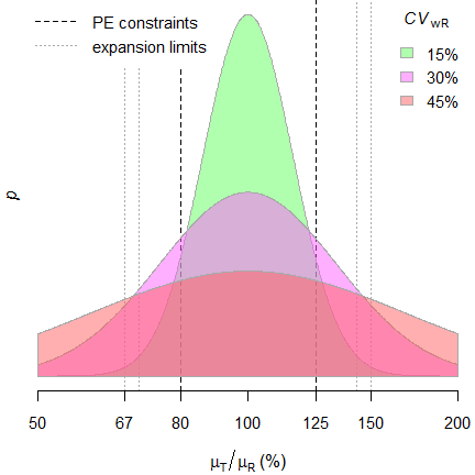
Since it is extremely unlikely that \(\small{s_\textrm{wR}\equiv
\sigma_\textrm{wR}}\), a drug / drug product may be
falsely classified as highly variable. Due to the scaled limits
the chance of passing increases compared to the correct
ABE.
Such a misclassificaton translates into an inflated Type I
Error (increased patient’s risk).
Contrary to ABE, where the fixed limits are based on a pre-specified clinically not relevant difference \(\small{\Delta}\), it is not surprising that the Type I Error may be inflated, since in SABE the clinically not relevant difference \(\small{\Delta}\) is unknown beforehand and the null hypothesis generated post hoc based on the \(\small{CV_{\textrm{wR}}}\) observed in the study. Consequently, the regulatory goalposts become random variables and each study sets its own rules, awarding ones with high variability.
Although in a particular study the realized clinically not
relevant difference \(\small{\widehat{\Delta}_\textrm{r}}\) can
be recalculated \[\widehat{\Delta}_\textrm{r}=100\,(1-\theta_{\textrm{s}_1})\tag{3}\]
but without access to the study report \(\small{\theta_{\textrm{s}_1}}\) is unknown
to physicians, pharmacists, and patients alike. Hence, this is an
unsatisfactory situation. We put the cart before the
horse.
Regrettably, apart from one anecdotal report,10 regulatory agencies
are paying little attention to the potentially increased consumer
risk.
Preliminaries
A basic knowledge of R is
required. To run the scripts at least version 1.4.8 (2019-08-29) of
PowerTOST is required and at least version 1.5.3
(2021-01-18) suggested. Any version of R would
likely do, though the current release of PowerTOST was only
tested with R-version 4.1.3 (2022-03-10) and
later. All scripts were run on a Xeon E3-1245v3 @ 3.40GHz (1/4 cores)
16GB RAM with R 4.2.2 on Windows 7 build 7601,
Service Pack 1, Universal C Runtime 10.0.10240.16390.
library(PowerTOST)          # attach it to run the examples
packs <- c("simcrossover", "adjustalpha")
if (sum(packs %in% rownames(installed.packages())) == 2) {
  lapply(packs, library, character.only = TRUE)
  adjustalpha.avail = TRUE  # use the packages in scripts
} else {
  adjustalpha.avail = FALSE # use hard-coded results in scripts
}
Except for Health Canada and the FDA (where a mixed-effects model is required) the recommended evaluation by an ANOVA11 assumes homoscedasticity (\(\small{s_{\textrm{wT}}^{2}\equiv s_{\textrm{wR}}^{2}}\)), which is – more often than not – wrong.
For a quick overview of the regulatory limits use the function
scABEL() – for once in percent according to the
guidelines.
df1 <- data.frame(regulator = "FDA", method = "RSABE",
                  CV = c(30, 50), L = NA_real_, U = NA_real_,
                  cap = c("lower", "  -  "))
for (i in 1:2) {
  df1[i, 4:5] <- sprintf("%.2f%%", 100 * scABEL(df1$CV[i] / 100,
                         regulator = "FDA"))
}
df1$CV <- sprintf("%.3f%%", df1$CV)
df2 <- data.frame(regulator = "EMA", method = "ABEL",
                  CV = c(30, 50),
                  L = NA_real_, U = NA_real_,
                  cap = c("lower", "upper"))
df3 <- data.frame(regulator = "HC", method = "ABEL",
                  CV = c(30, 57.382),
                  L = NA_real_, U = NA_real_,
                  cap = c("lower", "upper"))
for (i in 1:2) {
  df2[i, 4:5] <- sprintf("%.2f%%", 100 * scABEL(df2$CV[i] / 100))
  df3[i, 4:5] <- sprintf("%.1f %%", 100 * scABEL(df3$CV[i] / 100,
                         regulator = "HC"))
}
df2$CV <- sprintf("%.3f%%", df2$CV)
df3$CV <- sprintf("%.3f%%", df3$CV)
if (packageVersion("PowerTOST") >= "1.5.3") {
  df4 <- data.frame(regulator = "GCC", method = "ABEL",
                    CV = c(30, 50), L = NA_real_, U = NA_real_,
                    cap = c("lower", "  -  "))
  for (i in 1:2) {
    df4[i, 4:5] <- sprintf("%.2f%%", 100 * scABEL(df4$CV[i] / 100,
                           regulator = "GCC"))
  }
  df4$CV <- sprintf("%.3f%%", df4$CV)
}
if (packageVersion("PowerTOST") >= "1.5.3") {
  print(rbind(df1, df2, df3, df4), row.names = FALSE)
} else {
  print(rbind(df1, df2, df3), row.names = FALSE)
}
# regulator method CV L U cap
# FDA RSABE 30.000% 80.00% 125.00% lower
# FDA RSABE 50.000% 65.60% 152.45% -
# EMA ABEL 30.000% 80.00% 125.00% lower
# EMA ABEL 50.000% 69.84% 143.19% upper
# HC ABEL 30.000% 80.0 % 125.0 % lower
# HC ABEL 57.382% 66.7 % 150.0 % upper
# GCC ABEL 30.000% 80.00% 125.00% lower
# GCC ABEL 50.000% 75.00% 133.33% -Note that these are the ‘implied limits’ of RSABE. The FDA assesses the Type I Error based on the limits of the ‘desired consumer risk model’. More about that later.
Type I Error
Numerous authors observed an inflated TIE.13 14 15 16 17 18 19 20 21 22 23 24 25 26
In the following by ‘critical region’ I’m referring to the range of
\(\small{CV_\textrm{wR}}\)-values where
an inflated TIE is obtained in simulations.
Let’s explore an example: A four-period full replicate design in 24 subjects, \(\small{CV_{\textrm{wR}}=20-60\%}\). We perform one million simulations at the respective upper boundary of the equivalence range \(\small{\theta_{\textrm{s}_2}}\) (due to the symmetry in log-scale similar results are obtained at the lower boundary \(\small{\theta_{\textrm{s}_1}}\)). Because of the positive skewness of both \(\small{CV_{\textrm{wR}}}\) and \(\small{\theta_0}\), the upper boundary represents generally the worst case scenario.
The standard error of the empiric TIE is calculated according to \(\small{SE=\sqrt{0.5\cdot TIE_\textrm{emp}/10^6}}\). Starred values denote a significant inflation of the TIE based on the one-sided binomial test (> 0.05036).
CV     <- sort(c(seq(0.20, 0.50, 0.05),
                 se2CV(c(0.25, 0.294)), 0.60))
n      <- 24
design <- "2x2x4"
nsims  <- 1e6
sign.i <- binom.test(0.05*nsims, nsims, alternative = "less")$conf.int[2]
reg    <- c("FDA", "EMA", "HC")
if (packageVersion("PowerTOST") >= "1.5.3") reg <- c(reg, "GCC")
res    <- data.frame(regulator = rep(reg, each = length(CV)),
                     method = c(rep("RSABE", length(CV)),
                                rep("ABEL", (length(reg)-1)*length(CV))),
                     CVwR = CV, theta2 = NA, TIE.emp = NA,
                     SE = NA, infl = "")
for (i in 1:nrow(res)) {
  res$theta2[i] <- scABEL(res$CVwR[i],
                          regulator = res$regulator[i])[["upper"]]
  if (res$regulator[i] == "FDA") {
    res$TIE.emp[i] <- power.RSABE(CV = res$CVwR[i], design = design,
                                  theta0 = res$theta2[i], n = n,
                                  nsims = nsims)
}else {
    res$TIE.emp[i] <- power.scABEL(CV = res$CVwR[i], design = design,
                                   theta0 = res$theta2[i], n = n,
                                   nsims = nsims,
                                   regulator = res$regulator[i])
  }
  res$theta2[i] <- signif(res$theta2[i], 5)
  res$SE[i] <- sprintf("%.5f", sqrt(0.5 * res$TIE[i] / nsims))
  if (res$TIE[i] > sign.i) res$infl[i] <- "* "
}
res$CVwR    <- signif(res$CVwR, 5)
res$TIE.emp <- round(res$TIE.emp, 5)
print(res, row.names = FALSE)
# regulator method CVwR theta2 TIE.emp SE infl
# FDA RSABE 0.20000 1.2500 0.05023 0.00016
# FDA RSABE 0.25000 1.2500 0.06329 0.00018 *
# FDA RSABE 0.25396 1.2500 0.06634 0.00018 *
# FDA RSABE 0.30000 1.2500 0.13351 0.00026 *
# FDA RSABE 0.30047 1.3001 0.04782 0.00015
# FDA RSABE 0.35000 1.3545 0.04098 0.00014
# FDA RSABE 0.40000 1.4104 0.03071 0.00012
# FDA RSABE 0.45000 1.4671 0.02139 0.00010
# FDA RSABE 0.50000 1.5245 0.01455 0.00009
# FDA RSABE 0.60000 1.6404 0.00707 0.00006
# EMA ABEL 0.20000 1.2500 0.04994 0.00016
# EMA ABEL 0.25000 1.2500 0.05224 0.00016 *
# EMA ABEL 0.25396 1.2500 0.05312 0.00016 *
# EMA ABEL 0.30000 1.2500 0.08040 0.00020 *
# EMA ABEL 0.30047 1.2504 0.08014 0.00020 *
# EMA ABEL 0.35000 1.2948 0.06527 0.00018 *
# EMA ABEL 0.40000 1.3402 0.05944 0.00017 *
# EMA ABEL 0.45000 1.3859 0.04780 0.00015
# EMA ABEL 0.50000 1.4319 0.03289 0.00013
# EMA ABEL 0.60000 1.4319 0.04490 0.00015
# HC ABEL 0.20000 1.2500 0.05012 0.00016
# HC ABEL 0.25000 1.2500 0.05385 0.00016 *
# HC ABEL 0.25396 1.2500 0.05490 0.00017 *
# HC ABEL 0.30000 1.2500 0.08414 0.00021 *
# HC ABEL 0.30047 1.2504 0.08396 0.00020 *
# HC ABEL 0.35000 1.2948 0.06869 0.00019 *
# HC ABEL 0.40000 1.3402 0.06150 0.00018 *
# HC ABEL 0.45000 1.3859 0.05283 0.00016 *
# HC ABEL 0.50000 1.4319 0.04299 0.00015
# HC ABEL 0.60000 1.5000 0.03326 0.00013
# GCC ABEL 0.20000 1.2500 0.05026 0.00016
# GCC ABEL 0.25000 1.2500 0.07342 0.00019 *
# GCC ABEL 0.25396 1.2500 0.07838 0.00020 *
# GCC ABEL 0.30000 1.3333 0.02200 0.00010
# GCC ABEL 0.30047 1.3333 0.02219 0.00011
# GCC ABEL 0.35000 1.3333 0.03865 0.00014
# GCC ABEL 0.40000 1.3333 0.04608 0.00015
# GCC ABEL 0.45000 1.3333 0.04836 0.00016
# GCC ABEL 0.50000 1.3333 0.04896 0.00016
# GCC ABEL 0.60000 1.3333 0.04884 0.00016We see a huge inflation of the TIE in the
FDA’s
RSABE and
the GCC’s variant of
ABEL
up to the switching \(\small{C_\textrm{wR}}\) of 30%. Then the
TIE is controlled due the inherent conservatism of the
TOST and the
PE-constraint.
Note the discontinuity of the
GCC’s method because for
any \(\small{C_\textrm{wR}>30\%}\)
the limits are directly widened to 0.7500–1.3333.
ABEL for the EMA and Health Canada shows less inflation. However, it reaches beyond the switching \(\small{C_\textrm{wR}}\) of 30%. Due to the more liberal upper cap of scaling (≈57.4% instead of 50%) the inflation for Health Canada is slightly more pronounced than for the EMA. In either case, for large variabilities (> 45–50%) the TIE is controlled.
The TIE depends on the sample size as well. Simulations like above but with \(\small{n=24-48}\) at \(\small{CV_{\textrm{wR}}=30\%}\) (\(\small{\theta_{\textrm{s}_2}=1.25}\)); ABE for comparative purposes only.
CV     <- 0.30
n      <- seq(24, 48, 12)
design <- "2x2x4"
nsims  <- 1e6
sign.i <- binom.test(0.05*nsims, nsims, alternative = "less")$conf.int[2]
reg    <- c("all", "FDA", "EMA", "HC")
if (packageVersion("PowerTOST") >= "1.5.3") reg <- c(reg, "GCC")
res    <- data.frame(regulator = rep(reg, each = length(n)),
                     method = c(rep("ABE", length(n)),
                                rep("RSABE", length(n)),
                                rep("ABEL", (length(reg)-2)*length(n))),
                     n = n, TIE.emp = NA, SE = NA, infl = "")
for (i in 1:nrow(res)) {
  if (res$regulator[i] == "all") {
    theta1 <- 1.25
}else {
    theta2 <- scABEL(CV, regulator = res$regulator[i])[["upper"]]
  }
  if (res$regulator[i] == "FDA") {
    res$TIE.emp[i] <- power.RSABE(CV = CV, design = design,
                                  theta0 = theta2, n = res$n[i],
                                  nsims = nsims)
}else {
    if (res$regulator[i] == "all") {
      res$TIE.emp[i] <- power.TOST(CV = CV, design = design,
                                   theta0 = 1.25, n = res$n[i])
  }else {
      res$TIE.emp[i] <- power.scABEL(CV = CV, design = design,
                                     theta0 = theta2, n = res$n[i],
                                     nsims = nsims,
                                     regulator = res$regulator[i])
    }
  }
  res$SE[i] <- sprintf("%.5f", sqrt(0.5 * res$TIE[i] / nsims))
  if (res$TIE[i] > sign.i) res$infl[i] <- "* "
}
res$TIE.emp <- round(res$TIE.emp, 5)
print(res, row.names = FALSE)
# regulator method n TIE.emp SE infl
# all ABE 24 0.05000 0.00016
# all ABE 36 0.05000 0.00016
# all ABE 48 0.05000 0.00016
# FDA RSABE 24 0.13351 0.00026 *
# FDA RSABE 36 0.15360 0.00028 *
# FDA RSABE 48 0.17076 0.00029 *
# EMA ABEL 24 0.08040 0.00020 *
# EMA ABEL 36 0.08192 0.00020 *
# EMA ABEL 48 0.08232 0.00020 *
# HC ABEL 24 0.08414 0.00021 *
# HC ABEL 36 0.08461 0.00021 *
# HC ABEL 48 0.08465 0.00021 *
# GCC ABEL 24 0.14932 0.00027 *
# GCC ABEL 36 0.19307 0.00031 *
# GCC ABEL 48 0.23244 0.00034 *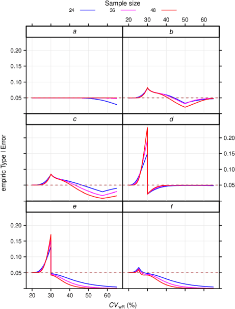
Fig. 2 Empiric TIE in
4-period full replicate designs.
a ABE, b ABEL
(EMA),
c ABEL (Health Canada), d ABEL
(GCC),
e RSABE (‘implied
limits’), f RSABE (‘desired consumer
risk model’)
Of course, in ABE the TIE is always controlled, i.e., it never exceeds nominal \(\small{\alpha}\). Since TOST is not a most powerful test,27 for high \(\small{C_\textrm{wR}}\) together with relatively low sample sizes, it becomes conservative. Again, the FDA’s RSABE and the GCC’s variant of ABEL behave similarly and show a substanial dependency on the sample size. The two other ABEL methods are less sensitive to the sample size in the critical region.
Combining what we have seen so far for ABE, the FDA’s RSABE, the EMA’s and Health Canada’s ABEL, as well as the GCC’s variant of ABEL in 2-sequence 4-period full replicate designs (n 20–120). The pink plane is at the nominal \(\small{\alpha=0.05}\):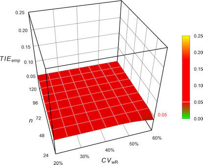
Fig. 3 Exact Type I Error of
ABE.
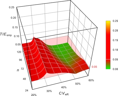
Fig. 4 Empiric Type I Error of
the EMA’s
ABEL.
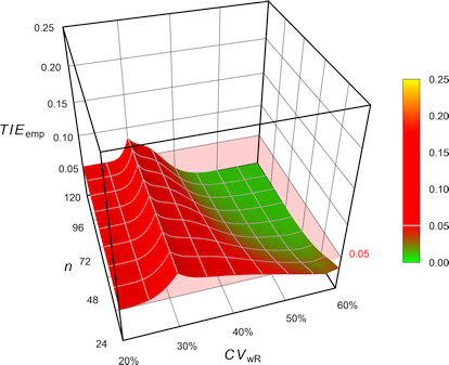
Fig. 5 Empiric Type I Error of
Health Canada’s
ABEL.
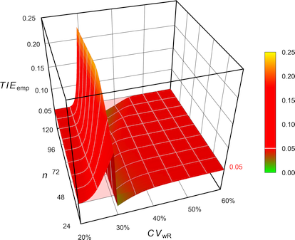
Fig. 6 Empiric Type I Error of
the GCC’s approach.
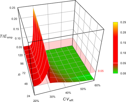
Fig. 7 Empiric Type I Error of
the FDA’s
RSABE.
The FDA assessed the Type I Error not at the ‘implied limits’ – like all [sic] other authors – but based on the limits of the so-called ‘desired consumer risk model’.28 29 \[\begin{array}{ll}\tag{4} \theta_0=1.25 & \textrm{if}\; s_\textrm{wR}<0.294,\\ \theta_0=\exp(\frac{\log_{e}1.25}{0.25}\cdot s_\textrm{wR}) & \textrm{otherwise}. \end{array}\]
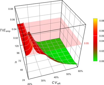
Fig. 8 Empiric Type I Error of
RSABE
according to the
FDA’s ‘desired
consumer risk model’.
Contrary to all other methods, where the TIE increases with the sample size, in the ‘desired consumer risk model’ the largest TIE is observed at small sample sizes.
Let’s explore that in 4-period full replicate studies with a T/R-ratio of 0.90 powered at 80%.
CV  <- CV  <- sort(c(seq(0.2, 0.4, 0.05), se2CV(0.25), 0.272645))
res <- data.frame(n = NA, CVwR = CV, swR = CV2se(CV),
                  impl.L = NA, impl.U = NA, impl.TIE = NA,
                  des.L = NA, des.U = NA, des.TIE = NA)
for (i in 1:nrow(res)) {
  res$n[i] <- sampleN.RSABE(CV = CV[i], design = "2x2x4",
                           details = FALSE,
                           print = FALSE)[["Sample size"]]
  res[i, 4:5] <- scABEL(CV = CV[i], regulator = "FDA")
  if (CV2se(CV[i]) <= 0.25) {
    res[i, 7:8] <- c(0.80, 1.25)
}else {
    res[i, 7:8] <- exp(c(-1, +1)*(log(1.25)/0.25)*CV2se(CV[i]))
  }
  res[i, 6]     <- power.RSABE(CV = CV[i], design = "2x2x4",
                               theta0 = res[i, 5], n = res$n[i],
                               nsims = 1e6)
  res[i, 9]     <- power.RSABE(CV = CV[i], design = "2x2x4",
                               theta0 = res[i, 8], n = res$n[i],
                               nsims = 1e6)
}
res[, 2:3] <- round(res[, 2:3], 3)
res[, c(4:5, 7:8)] <- round(res[, c(4:5, 7:8)], 4)
res[, c(6, 9)] <- round(res[, c(6, 9)], 5)
print(res, row.names = FALSE)
# n CVwR swR impl.L impl.U impl.TIE des.L des.U des.TIE
# 20 0.200 0.198 0.8000 1.2500 0.05047 0.8000 1.2500 0.05047
# 28 0.250 0.246 0.8000 1.2500 0.06195 0.8000 1.2500 0.06195
# 30 0.254 0.250 0.8000 1.2500 0.06467 0.8000 1.2500 0.06467
# 32 0.273 0.268 0.8000 1.2500 0.08783 0.7874 1.2700 0.05000
# 32 0.300 0.294 0.8000 1.2500 0.14714 0.7695 1.2996 0.04611
# 28 0.350 0.340 0.7383 1.3545 0.03923 0.7383 1.3545 0.03923
# 24 0.400 0.385 0.7090 1.4104 0.03071 0.7090 1.4104 0.03071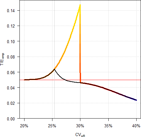
Fig. 9 Empiric Type I Error in a
4-period full replicate design (n 32).
Colored line ‘implied
limits’, black line ‘desired consumer risk model’.
In my opinion the ‘desired consumer risk model’ is nothing more than a mathematical prestidigitation as drug products are not approved according its conditions but the ones of the guidances.30 31 Some eminent statisticians32 call it just a hocus pocus…
Remedies?
In the following 3D-plots the z-axis is scaled to the maximum of the empiric Type I Error for the EMA’s ABEL (0.084392).
Ad hoc
Bonferroni
Whilst seemingly obvious, it is problematic for numerous reasons.
- It is not known beforehand how many decisions and tests k will be performed in the
regulatory frameworks and hence, any adjustment arbitrary.
- RSABE
- swR ≥ 0.294
- If the upper critical bound is ≤ 0, assess the PE (within the constraints 80.00–125.00%).
- swR <
0.294
- Assess the 90% CI for ABE.
- swR ≥ 0.294
- ABEL
- CVwR >
30%
- If CVwR ≤ 50% use swR for expanding the limits or the upper cap, otherwise.
- If the 90% CI is within the expanded limits, assess the PE (within the constraints 80.00–125.00%).
- CVwR ≤ 30%
- Assess the 90% CI for ABE.
- CVwR >
30%
- RSABE
- The tests are not independent.
- The approach is overly conservative if an inflated TIE is unlikely (say, if CVwR > 45% in ABEL and if CVwR < 30% in RSABE).
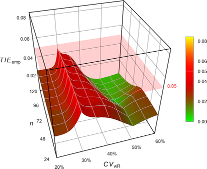
Fig. 10 Empiric Type I Error of
the EMA’s
ABEL
with Bonferroni’s \(\small{\alpha=0.025}\).
CVwR   <- 0.35
design <- "2x2x4"
theta0 <- 0.90
tmp    <- sampleN.scABEL(CV = CVwR, theta0 = theta0,
                         design = design, details = FALSE,
                         print = FALSE)
cat("Design        ", design,
    "\nMethod         ABEL (EMA)",
    "\nCVwR          ", CVwR,
    "\ntheta0        ", theta0,
    "\nSample size   ", tmp[["Sample size"]],
    "\nAchieved power", tmp[["Achieved power"]], "\n\n")
scABEL.ad(alpha.pre = 0.05 / 2, CV = CVwR, theta0 = theta0,
          design = design, n = tmp[["Sample size"]],
          details = TRUE)
# Design 2x2x4
# Method ABEL (EMA)
# CVwR 0.35
# theta0 0.9
# Sample size 34
# Achieved power 0.81184
#
# +++++++++++ scaled (widened) ABEL ++++++++++++
# iteratively adjusted alpha
# (simulations based on ANOVA evaluation)
# ----------------------------------------------
# Study design: 2x2x4 (4 period full replicate)
# log-transformed data (multiplicative model)
# 1,000,000 studies in each iteration simulated.
#
# CVwR 0.35, CVwT 0.35, n(i) 17|17 (N 34)
# Nominal alpha : 0.05, pre-specified alpha 0.025
# True ratio : 0.9000
# Regulatory settings : EMA (ABEL)
# Switching CVwR : 0.3
# Regulatory constant : 0.76
# Expanded limits : 0.7723 ... 1.2948
# Upper scaling cap : CVwR > 0.5
# PE constraints : 0.8000 ... 1.2500
# Empiric TIE for alpha 0.0250 : 0.03614 (rel. change of risk: -27.7%)
# Power for theta0 0.9000 : 0.722
# TIE = nominal alpha; the chosen pre-specified alpha is justified.With \(\small{\alpha_{\textrm{adj}}=0.05/2}\) the TIE is controlled. However, the sample size has to be increased (in this example by ~24%) in order to maintain the target power.
- In some extreme cases it leads still to an inflated TIE:
CVwR   <- 0.30
design <- "2x2x3"
theta0 <- 0.85
Bonf   <- 0.05 / 2
n      <- sampleN.scABEL(alpha = Bonf, CV = CVwR, theta0 = theta0,
                         design = design, print = FALSE,
                         details = FALSE)[["Sample size"]]
scABEL.ad(alpha.pre = Bonf, CV = CVwR, theta0 = theta0,
          design = design, n = n)
# +++++++++++ scaled (widened) ABEL ++++++++++++
# iteratively adjusted alpha
# (simulations based on ANOVA evaluation)
# ----------------------------------------------
# Study design: 2x2x3 (3 period full replicate)
# log-transformed data (multiplicative model)
# 1,000,000 studies in each iteration simulated.
#
# CVwR 0.3, CVwT 0.3, n(i) 120|120 (N 240)
# Nominal alpha : 0.05, pre-specified alpha 0.025
# True ratio : 0.8500
# Regulatory settings : EMA (ABE)
# Switching CVwR : 0.3
# BE limits : 0.8000 ... 1.2500
# Upper scaling cap : CVwR > 0.5
# PE constraints : 0.8000 ... 1.2500
# Empiric TIE for alpha 0.0250 : 0.05243
# Power for theta0 0.8500 : 0.800
# Iteratively adjusted alpha : 0.02356
# Empiric TIE for adjusted alpha: 0.05000
# Power for theta0 0.8500 : 0.793Muñoz et al.
Muñoz et al.18 proposed to apply Howe’s approximation34 (like in RSABE) but according to the EMA’s conditions (regulatory constant 0.760, upper cap of scaling 50%).
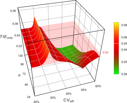
Fig. 11 Empiric Type I Error of
the EMA’s
ABEL
with Howe’s approximation.
# Cave: Long runtime
CV     <- 0.30
n      <- sampleN.scABEL(CV = CV, design = "2x2x4",
                         details = FALSE,
                         print = FALSE)[["Sample size"]]
CV     <- sort(c(se2CV(0.294),
                 seq(0.15, 0.65, 0.005)))
comp   <- data.frame(method = rep(c("EMA (2010)",
                                    "Muñoz et al. (2016)"),
                                  each = length(CV)),
                     CV = CV, TIE = NA)
theta2 <- rep(scABEL(CV = CV, regulator = "EMA")[, "upper"], 2)
for (i in 1:nrow(comp)) {
  if (comp$method[i] == "EMA (2010)") {
    comp$TIE[i] <- power.scABEL(CV = comp$CV[i], n = n,
                                design = "2x2x4",
                                theta0 = theta2[i],
                                nsims = 1e6)
}else {
    comp$TIE[i] <- power.RSABE(CV = comp$CV[i], n = n,
                               design = "2x2x4",
                               theta0 = theta2[i],
                               regulator = "EMA",
                               nsims = 1e6)
  }
}
dev.new(width = 4.5, height = 4.5)
op   <- par(no.readonly = TRUE)
par(mar = c(4, 3.9, 0.1, 0.1), cex.axis = 0.9)
ylim <- c(0, max(comp$TIE))
xlim <- c(0.2, 0.6)
plot(CV, comp$TIE[comp$method == "EMA (2010)"], type = "n",
     xlab = expression(italic(CV)[wR]), xlim = xlim, ylim = ylim,
     ylab = "empiric Type I Error", axes = FALSE)
grid()
abline(v = c(0.3, 0.5), lty = 2)
abline(h = 0.05)
axis(1, at = pretty(CV),
     labels = sprintf("%i%%", as.integer(100*pretty(CV))))
axis(2, las = 1)
legend("bottomleft",
       legend = c("EMA (2010)",
                  expression("Muñoz "*italic("et al")*". (2016)")),
       col = c("#FF000080", "#FF00FF80"),
       lwd = 3, cex = 0.9, box.lty = 0, bg = "white", inset = 0.02)
box()
lines(CV, comp$TIE[comp$method == "EMA (2010)"],
      lwd = 3, col = "#FF000080")
lines(CV, comp$TIE[comp$method == "Muñoz et al. (2016)"],
      lwd = 3, col = "#FF00FF80")
par(op)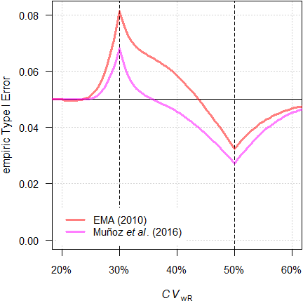
Fig. 12 TIE of the
approaches in a 4-period full replicate design (n 34).
We see less inflation of the TIE (its maximum decreases from 0.0816 to 0.0684) and the critical region is substantially narrower. Whilst this is an improvement over the original method, it is not considered further.
Labes and Schütz

Fig. 13 Empiric Type I Error of
the EMA’s
ABEL
when assessed with iteratively adjusted \(\small{\alpha}\).
CVwR   <- 0.35
design <- "2x2x4"
theta0 <- 0.90
tmp    <- sampleN.scABEL(CV = CVwR, theta0 = theta0,
                         design = design, details = FALSE,
                         print = FALSE)
cat("Design        ", design,
    "\nMethod         ABEL (EMA)",
    "\nCVwR          ", CVwR,
    "\ntheta0        ", theta0,
    "\nSample size   ", tmp[["Sample size"]],
    "\nAchieved power", tmp[["Achieved power"]], "\n\n")
scABEL.ad(CV = CVwR, theta0 = theta0,
          design = design, n = tmp[["Sample size"]],
          details = TRUE)
# Design 2x2x4
# Method ABEL (EMA)
# CVwR 0.35
# theta0 0.9
# Sample size 34
# Achieved power 0.81184
#
# +++++++++++ scaled (widened) ABEL ++++++++++++
# iteratively adjusted alpha
# (simulations based on ANOVA evaluation)
# ----------------------------------------------
# Study design: 2x2x4 (4 period full replicate)
# log-transformed data (multiplicative model)
# 1,000,000 studies in each iteration simulated.
#
# CVwR 0.35, CVwT 0.35, n(i) 17|17 (N 34)
# Nominal alpha : 0.05
# True ratio : 0.9000
# Regulatory settings : EMA (ABEL)
# Switching CVwR : 0.3
# Regulatory constant : 0.76
# Expanded limits : 0.7723 ... 1.2948
# Upper scaling cap : CVwR > 0.5
# PE constraints : 0.8000 ... 1.2500
# Empiric TIE for alpha 0.0500 : 0.06557 (rel. change of risk: +31.1%)
# Power for theta0 0.9000 : 0.812
# Iteratively adjusted alpha : 0.03630
# Empiric TIE for adjusted alpha: 0.05000
# Power for theta0 0.9000 : 0.773 (rel. impact: -4.81%)
#
# Runtime : 6.76 seconds
# Simulations: 7,100,000 (6 iterations)With \(\small{\alpha_{\textrm{adj}}=0.0363}\) the
TIE is controlled. However, we loose some power. We can
counteract that in designing the study by means of the function
sampleN.scABEL.ad().
CVwR   <- 0.35
design <- "2x2x4"
theta0 <- 0.90
sampleN.scABEL.ad(CV = CVwR, theta0 = theta0,
                  design = design)
#
# +++++++++++ scaled (widened) ABEL ++++++++++++
# Sample size estimation
# for iteratively adjusted alpha
# (simulations based on ANOVA evaluation)
# ----------------------------------------------
# Study design: 2x2x4 (4 period full replicate)
# log-transformed data (multiplicative model)
# 1,000,000 studies in each iteration simulated.
#
# Assumed CVwR 0.35, CVwT 0.35
# Nominal alpha : 0.05
# True ratio : 0.9000
# Target power : 0.8
# Regulatory settings: EMA (ABEL)
# Switching CVwR : 0.3
# Regulatory constant: 0.76
# Expanded limits : 0.7723 ... 1.2948
# Upper scaling cap : CVwR > 0.5
# PE constraints : 0.8000 ... 1.2500
# n 38, adj. alpha: 0.03610 (power 0.8100), TIE: 0.05000We need a ~12% larger sample size.
Similarly for RSABE, where we expect an inflated TIE for \(\small{CV_\textrm{wR}<30\%}\). This time spiced with heteroscedasticity (\(\small{CV_\textrm{wR}>CV_\textrm{wT}}\)).
CVw    <- 0.25
CVw    <- signif(CVp2CV(0.25, ratio = 0.80), 4)
design <- "2x2x4"
theta0 <- 0.90
tmp    <- sampleN.RSABE(CV = CVw, theta0 = theta0,
                        design = design, details = FALSE,
                        print = FALSE)
cat("Design        ", design,
    "\nMethod         RSABE (FDA)",
    "\nCVw (R, T)    ", paste(sprintf("%.4f", rev(CVw)), collapse = ", "),
    "\ntheta0        ", theta0,
    "\nSample size   ", tmp[["Sample size"]],
    "\nAchieved power", tmp[["Achieved power"]], "\n\n")
scABEL.ad(CV = CVw, theta0 = theta0,
          design = design, n = tmp[["Sample size"]],
          regulator = "FDA", details = FALSE)
# Design 2x2x4
# Method RSABE (FDA)
# CVw (R, T) 0.2640, 0.2353
# theta0 0.9
# Sample size 28
# Achieved power 0.81882
#
# +++++++++++ scaled (widened) ABEL ++++++++++++
# iteratively adjusted alpha
# (simulations based on intra-subject contrasts)
# ----------------------------------------------
# Study design: 2x2x4 (4 period full replicate)
# log-transformed data (multiplicative model)
# 1,000,000 studies in each iteration simulated.
#
# CVwR 0.264, CVwT 0.2353, n(i) 14|14 (N 28)
# Nominal alpha : 0.05
# True ratio : 0.9000
# Regulatory settings : FDA (ABE)
# Switching CVwR : 0.3
# BE limits : 0.8000 ... 1.2500
# PE constraints : 0.8000 ... 1.2500
# Empiric TIE for alpha 0.0500 : 0.07697
# Power for theta0 0.9000 : 0.819
# Iteratively adjusted alpha : 0.03053
# Empiric TIE for adjusted alpha: 0.05000
# Power for theta0 0.9000 : 0.747- The method has to be stated in the protocol. No problems are expected from authorities. Even if an assessor doesn’t believe [sic] in an inflated TIE, there are no reasons to object using an apparently more conservative α.
- State not only the adjusted α (which is based on an assumed CVwR and the planned sample size) but make clear that in the study it will be recalculated based on the observed CVwR and actual sample size.
Molins et al.
Molins et al.22 argued that the true \(\small{\sigma_\textrm{wR}}\) is unknown, i.e., questioned the assumption of \(\small{s_\textrm{wR}=\sigma_\textrm{wR}}\) by Labes and Schütz.19 Hence, the authors proposed to adjust \(\small{\alpha}\) always for the worst case \(\small{CV_\textrm{wR}=30\%}\), where the largest inflation of the TIE is expected in ABEL.
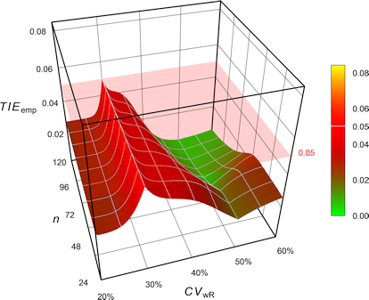
Fig. 14 Empiric Type I Error of
the EMA’s
ABEL
when assessed with iteratively adjusted \(\small{\alpha}\)
for
CVwR 30% irrespective of the observed
CVwR.
While reasonable, such a conservatism comes with a price.26 The sample size has to be increased even if an inflated TIE is unlikely (say, for \(\small{CV_\textrm{wR}\geq 45\%}\)).
CVwR   <- 0.50
design <- "2x2x4"
theta0 <- 0.90
tmp    <- sampleN.scABEL(CV = CVwR, theta0 = theta0,
                         design = design, details = FALSE,
                         print = FALSE)
ad     <- scABEL.ad(CV = 0.30, # worst case
                    n = tmp$n,
                    design = design,
                    theta0 = theta0,
                    print = FALSE)
power  <- power.scABEL(alpha = ad$alpha.adj,
                       CV = CVwR,
                       n = tmp$n,
                       design = design,
                       theta0 = theta0)
cat("Design        ", design,
    "\nMethod         ABEL (Molins et al. 2017)",
    "\nCVwR          ", CVwR,
    "\ntheta0        ", theta0,
    "\nSample size   ", tmp[["Sample size"]],
    "\nAdjusted alpha", ad$alpha.adj, "(based on CVwR 0.30)",
    "\nEmpiric TIE   ", ad$TIE.adj,
    "\nAchieved power", power)
# Design 2x2x4
# Method ABEL (Molins et al. 2017)
# CVwR 0.5
# theta0 0.9
# Sample size 28
# Adjusted alpha 0.028865 (based on CVwR 0.30)
# Empiric TIE 0.05
# Achieved power 0.74063- The method has to be stated in the protocol. No problems are expected from authorities. Even if an assessor doesn’t believe [sic] in an inflated TIE, there are no reasons to object using an apparently more conservative α.
- State not only the adjusted α (which is based on the planned sample size) but make clear that in the study it will be recalculated based on the actual sample size. If there are dropouts, slightly less adjustment will be required.
Ocaña and Muñoz
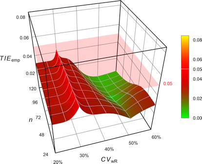
Fig. 15 Empiric Type I Error of
the EMA’s
ABEL
with Howe’s approximation when assessed
with iteratively adjusted
\(\small{\alpha}\) for
CVwR 30% irrespective of the observed
CVwR.
For the example above one gets an adjusted \(\small{\alpha}\) of 0.032407, which is less conservative than the one of Molins et al.22 (0.028865). Whilst the method controls the Type I Error, it leads to loss in power.
The R package adjustalpha can
be obtained from the authors.
‘Exact’
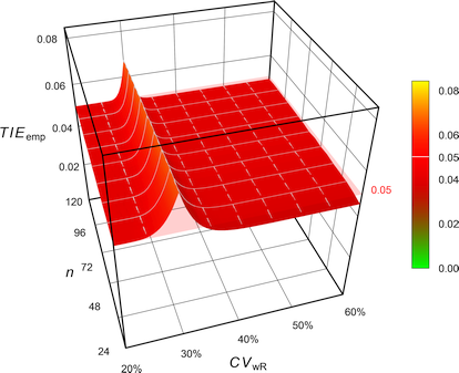
Fig. 16 Empiric Type I Error of
‘pure’
ABEL.
# 'Pure' EMA settings (without upper cap of expansion
# and PE constraint)
reg           <- reg_const("EMA")
reg$CVcap     <- Inf
reg$pe_constr <- FALSE
reg$name      <- "pure EMA"
# Cave: Subject data simulations = extremely long runtime
CV     <- 0.30
n      <- sampleN.scABEL(CV = CV, design = "2x2x4",
                         details = FALSE,
                         print = FALSE)[["Sample size"]]
CV     <- sort(c(se2CV(0.294),
                 seq(0.15, 0.65, 0.005)))
comp   <- data.frame(method = rep(c("EMA (2010)",
                                    "exact"),
                                  each = length(CV)),
                     CV = CV, TIE = NA)
theta2 <- c(scABEL(CV = CV, regulator = "EMA")[, "upper"],
            scABEL(CV = CV, regulator = reg)[, "upper"])
for (i in 1:nrow(comp)) {
  if (comp$method[i] == "EMA (2010)") {
    comp$TIE[i] <- power.scABEL(CV = comp$CV[i], n = n,
                                design = "2x2x4",
                                theta0 = theta2[i],
                                nsims = 1e6)
  }
  if (comp$method[i] == "exact") {
    comp$TIE[i] <- power.RSABE2L.sdsims(CV = comp$CV[i], n = n,
                                        design = "2x2x4",
                                        theta0 = theta2[i],
                                        regulator = reg,
                                        SABE_test = "exact",
                                        nsims = 1e6,
                                        progress = FALSE)
  }
  setTxtProgressBar(pb, i/nrow(comp))
}
dev.new(width = 4.5, height = 4.5, record = TRUE)
op   <- par(no.readonly = TRUE)
par(mar = c(4, 3.9, 0.1, 0.1), cex.axis = 0.9)
ylim <- c(0, max(comp$TIE))
xlim <- c(0.2, 0.6)
plot(CV, comp$TIE[comp$method == "EMA (2010)"], type = "n",
     xlab = expression(italic(CV)[wR]), xlim = xlim, ylim = ylim,
     ylab = "empiric Type I Error", axes = FALSE)
grid()
abline(v = c(0.3, 0.5), lty = 2)
abline(h = 0.05)
axis(1, at = pretty(CV),
     labels = sprintf("%i%%", as.integer(100*pretty(CV))))
axis(2, las = 1)
legend("bottomleft",
       legend = c("EMA (2010)",
                  "Tóthfalusi & Endrényi (2017)"),
       col = c("#FF000080", "#FF00FF80"),
       lwd = 3, cex = 0.9, box.lty = 0, bg = "white", inset = 0.02)
box()
lines(CV, comp$TIE[comp$method == "EMA (2010)"],
      lwd = 3, col = "#FF000080")
lines(CV, comp$TIE[comp$method == "exact"],
      lwd = 3, col = "#FF00FF80")
par(op)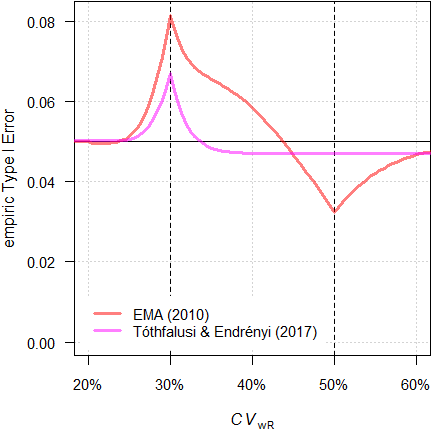
Fig. 17 Empiric TIE of
the approaches in a 4-period full replicate design (n 34).
With a maximum TIE of 0.0671 it performs better than the original ABEL (0.0816) and similarly to Muñoz et al.18 (0.0684). Furthermore, its critical region is slightly narrower (inflated TIE with \(\small{CV_\textrm{wR}}\) up to 33.7% vs 35.7%).
The authors discussed a combination with the iterative adjustment proposed by Labes and Schütz19 in the critical region, which would provide a smaller sample size penalty.
# Extremely (!) long runtime due to subject data
# simulations and potential iterative alpha-adjustment
limits <- function(CV, regulator) {
  thetas        <- scABEL(CV = CV, regulator = regulator)
  names(thetas) <- c("lower", "upper")
  return(thetas)
}
check.TIE <- function(alpha = 0.05, CV, n, design,
                      regulator) {
  thetas <- limits(CV = CV, regulator = regulator)
  power.RSABE2L.sdsims(CV = CV, n = n,
                       theta0 = theta2,
                       design = design,
                       regulator = regulator,
                       SABE_test = "exact",
                       nsims = 1e6,
                       progress = FALSE)
}
check.power <- function(alpha = 0.05, CV, n, design,
                        theta0, regulator) {
  thetas <- limits(CV = CV, regulator = regulator)
  power.RSABE2L.sdsims(CV = CV, n = n,
                       theta0 = theta0,
                       design = design,
                       regulator = regulator,
                       SABE_test = "exact")
}
opt <- function(x) {
  power.RSABE2L.sdsims(alpha = x, CV = CV, n = n,
                       theta0 = theta2, design = design,
                       regulator = reg,
                       SABE_test = "exact", nsims = 1e6,
                       progress = FALSE) - alpha
}
# 'Pure' EMA settings (without upper cap of expansion
# and PE constraint)
reg           <- reg_const("EMA")
reg$CVcap     <- Inf
reg$pe_constr <- FALSE
reg$name      <- "pure EMA"
alpha         <- 0.05
CV            <- 0.35
theta0        <- 0.90
design        <- "2x2x4"
target        <- 0.80
theta2        <- scABEL(CV = CV, regulator = reg)[["upper"]]
step          <- as.integer(substr(design, 3, 3))
alpha.adj     <- NA
iter          <- 0
# start with Muñoz' approach
n             <- sampleN.RSABE(CV = CV, design = design,
                               theta0 = theta0,
                               targetpower = target,
                               regulator = "EMA",
                               details = FALSE,
                               print = FALSE)[["Sample size"]]
TIE           <- check.TIE(CV = CV, n = n, design = design,
                           regulator = reg)
power         <- check.power(CV = CV, n = n, design = design,
                             theta0 = theta0,
                             regulator = reg)
res           <- data.frame(iter = iter, n = n,
                            alpha.adj = NA,
                            TIE = TIE, power = power)
if (TIE > alpha) {# inflated TIE with first guess n
   iter      <- iter + 1
   theta2    <- limits(CV = CV,
                       regulator = regulator)[["upper"]]
   x         <- uniroot(opt, interval = c(0.025, alpha),
                        tol = 1e-8)
   alpha.adj <- x$root
   TIE       <- x$f.root + alpha
   power     <- check.power(alpha = alpha.adj,
                            CV = CV, n = n,
                            design = design,
                            theta0 = theta0,
                            regulator = reg)
   res[iter+1, ] <- c(iter, n, alpha.adj, TIE, power)
} else {          # TIE OK, try a lower sample size
  repeat {
    iter  <- iter + 1
    n     <- n - step
    power <- check.power(CV = CV, n = n,
                         design = design,
                         theta0 = theta0,
                         regulator = reg)
    TIE   <- check.TIE(CV = CV, n = n,
                       design = design,
                       regulator = reg)
    if (TIE > alpha) {
      x         <- uniroot(opt, interval = c(0.025, alpha),
                           tol = 1e-8)
      alpha.adj <- x$root
      TIE       <- x$f.root + alpha
    }
    res[iter+1, ] <- c(iter, n, alpha.adj, TIE, power)
    if (power >= target) {
      break
    }
  }
}
est  <- max(which(res$n == min(res$n) &
                  res$power >= target))
txt1 <- paste("Sample size   ", res$n[est],
              "\nAchieved power", res$power[est])
txt2 <- paste("\nEmpiric TIE   ", res$TIE[est], "\n")
if (is.na(res$alpha[est])) {
  cat(paste(txt1, "\nAlpha         ", alpha), txt2)
} else {
  cat(paste(txt1, "\nAdjusted alpha",
            signif(res$alpha.adj[est], 4),
            txt2))
}
In the example above we would need no \(\small{\alpha}\)-adjustment because the \(\small{CV_\textrm{wR}}\) is above the critical region. With a sample size of 36 (TIE 0.0486) we need two subjects less than by the approach of Labes and Schütz.19
Its implementation would require a major revision of the regulatory approach. Although statistically appealing, it will currently not be accepted by regulatory agencies.
Comparison
Let’s estimate the sample size for the original ABEL and compare power and the empiric Type I Error of the remedies.
- \(\small{CV_\textrm{wR}=24\%}\), where we expect only a slight inflation of the TIE with the original ABEL.
CVwR   <- 0.24
design <- "2x2x4"
theta0 <- 0.90
tmp    <- sampleN.scABEL(CV = CVwR, theta0 = theta0,
                         design = design, details = FALSE,
                         print = FALSE)
info   <- paste("Design     ", design,
                "\nMethod      ABEL (EMA)",
                "\nCVwR       ", CVwR,
                "\ntheta0     ", theta0,
                "\nSample size", tmp[["Sample size"]], "\n")
comp   <- data.frame(method = c("EMA (2010)",
                                "Bonferroni (1936)",
                                "Muñoz et al (2016)",
                                "Labes and Schütz (2016)",
                                "Molins et al. (2017)",
                                "Tóthfalusi and Endrényi (2017)",
                                "Ocaña and Muñoz (2019)"),
                     adj = " \u2013 ", alpha = 0.05,
                     TIE.emp = NA, power = NA)
for (i in 1:nrow(comp)) {
  if (comp$method[i] == "EMA (2010)") {
    res <- scABEL.ad(CV = CVwR, n = tmp$n,
                     theta0 = theta0,
                     design = design,
                     print = FALSE)
    comp$TIE.emp[i] <- res$TIE.unadj
    comp$power[i]   <- res$pwr.unadj
  }
  if (comp$method[i] == "Bonferroni (1936)") {
    res <- scABEL.ad(alpha.pre = 0.05 / 2,
                     CV = CVwR, n = tmp$n,
                     theta0 = theta0,
                     design = design,
                     print = FALSE)
    comp$adj[i]     <- "yes"
    comp$alpha[i]   <- res$alpha.pre
    comp$TIE.emp[i] <- res$TIE.unadj
    comp$power[i]   <- res$pwr.unadj
  }
  if (comp$method[i] == "Muñoz et al (2016)") {
    comp$adj[i]     <- "no"
    comp$TIE.emp[i] <- power.RSABE(CV = CVwR,
                                   n = tmp$n,
                                   design = design,
                                   theta0 = scABEL(CV = CVwR)[["upper"]],
                                   regulator = "EMA")
    comp$power[i]   <- power.RSABE(CV = CVwR,
                                   n = tmp$n,
                                   design = design,
                                   theta0 = theta0,
                                   regulator = "EMA")
  }
  if (comp$method[i] == "Labes and Schütz (2016)") {
    res <- scABEL.ad(CV = CVwR, n = tmp$n,
                     theta0 = theta0,
                     design = design,
                     print = FALSE)
    if (is.na(res$alpha.adj)) {
      comp$adj[i]     <- "no"
      comp$alpha[i]   <- res$alpha
      comp$TIE.emp[i] <- res$TIE.unadj
      comp$power[i]   <- res$pwr.unadj
}else {
      comp$adj[i]     <- "yes"
      comp$alpha[i]   <- res$alpha.adj
      comp$TIE.emp[i] <- res$TIE.adj
      comp$power[i]   <- res$pwr.adj
    }
  }
  if (comp$method[i] == "Molins et al. (2017)") {
    res <- scABEL.ad(CV = 0.30, n = tmp$n,
                     theta0 = theta0,
                     design = design,
                     print = FALSE)
    comp$adj[i]     <- "yes"
    comp$alpha[i]   <- res$alpha.adj
    comp$TIE.emp[i] <- power.scABEL(alpha = res$alpha.adj,
                                    CV = CVwR,
                                    n = tmp$n,
                                    design = design,
                                    theta0 = scABEL(CV = CVwR)[["upper"]])
    comp$power[i]   <- power.scABEL(alpha = res$alpha.adj,
                                    CV = CVwR,
                                    n = tmp$n,
                                    design = design,
                                    theta0 = theta0)
  }
  if (comp$method[i] == "Tóthfalusi and Endrényi (2017)") {
    reg             <- reg_const("EMA")
    reg$CVcap       <- Inf
    reg$pe_constr   <- FALSE
    reg$name        <- "pure EMA"
    comp$adj[i]     <- "no"
    comp$TIE.emp[i] <- power.RSABE2L.sds(CV = CVwR,
                                         n = tmp$n,
                                         design = design,
                                         regulator = reg,
                                         theta0 = scABEL(CV = CVwR,
                                                         regulator = reg)[["upper"]])
    comp$power[i]   <- power.RSABE2L.sds(CV = CVwR,
                                         n = tmp$n,
                                         design = design,
                                         regulator = reg,
                                         theta0 = theta0)
  }
  if (comp$method[i] == "Ocaña and Muñoz (2019)") {
    if (adjustalpha.avail) {
      comp$alpha[i] <- adjAlpha(n = tmp$n, beMethod = "HoweEMA",
                                design =  "TRTR-RTRT", nsim = 1e6,
                                seed = 123456)
  }else {
      comp$alpha[i] <- 0.03255385 # hard-coded
    }
    if (comp$alpha[i] < 0.05) comp$adj[i] <- "yes"
    comp$TIE.emp[i] <- power.RSABE(alpha = comp$alpha[i],
                                   CV = CVwR,
                                   n = tmp$n,
                                   design = design,
                                   theta0 = scABEL(CV = CVwR)[["upper"]],
                                   regulator = "EMA")
    comp$power[i]   <- power.RSABE(alpha = comp$alpha[i],
                                   CV = CVwR,
                                   n = tmp$n,
                                   design = design,
                                   theta0 = theta0,
                                   regulator = "EMA")
  }
}
comp[, 3:5] <- signif(comp[, 3:5], 4)
cat(info)
print(comp, row.names = FALSE, right = FALSE)
# Design 2x2x4
# Method ABEL (EMA)
# CVwR 0.24
# theta0 0.9
# Sample size 26
# method adj alpha TIE.emp power
# EMA (2010) – 0.05000 0.05054 0.8109
# Bonferroni (1936) yes 0.02500 0.02502 0.7116
# Muñoz et al (2016) no 0.05000 0.04997 0.7946
# Labes and Schütz (2016) yes 0.04951 0.05000 0.8096
# Molins et al. (2017) yes 0.02914 0.02919 0.7348
# Tóthfalusi and Endrényi (2017) no 0.05000 0.05054 0.8066
# Ocaña and Muñoz (2019) yes 0.03255 0.03229 0.7270- \(\small{CV_\textrm{wR}=30\%}\), where we expect the maximum TIE with the original ABEL.
CVwR   <- 0.30
design <- "2x2x4"
theta0 <- 0.90
tmp    <- sampleN.scABEL(CV = CVwR, theta0 = theta0,
                         design = design, details = FALSE,
                         print = FALSE)
info   <- paste("Design     ", design,
                "\nMethod      ABEL (EMA)",
                "\nCVwR       ", CVwR,
                "\ntheta0     ", theta0,
                "\nSample size", tmp[["Sample size"]], "\n")
comp   <- data.frame(method = c("EMA (2010)",
                                "Bonferroni (1936)",
                                "Muñoz et al (2016)",
                                "Labes and Schütz (2016)",
                                "Molins et al. (2017)",
                                "Tóthfalusi and Endrényi (2017)",
                                "Ocaña and Muñoz (2019)"),
                     adj = " \u2013 ", alpha = 0.05,
                     TIE.emp = NA, power = NA)
for (i in 1:nrow(comp)) {
  if (comp$method[i] == "EMA (2010)") {
    res <- scABEL.ad(CV = CVwR, n = tmp$n,
                     theta0 = theta0,
                     design = design,
                     print = FALSE)
    comp$TIE.emp[i] <- res$TIE.unadj
    comp$power[i]   <- res$pwr.unadj
  }
  if (comp$method[i] == "Bonferroni (1936)") {
    res <- scABEL.ad(alpha.pre = 0.05 / 2,
                     CV = CVwR, n = tmp$n,
                     theta0 = theta0,
                     design = design,
                     print = FALSE)
    comp$adj[i]     <- "yes"
    comp$alpha[i]   <- res$alpha.pre
    comp$TIE.emp[i] <- res$TIE.unadj
    comp$power[i]   <- res$pwr.unadj
  }
  if (comp$method[i] == "Muñoz et al (2016)") {
    comp$adj[i]     <- "no"
    comp$TIE.emp[i] <- power.RSABE(CV = CVwR,
                                   n = tmp$n,
                                   design = design,
                                   theta0 = scABEL(CV = CVwR)[["upper"]],
                                   regulator = "EMA")
    comp$power[i]   <- power.RSABE(CV = CVwR,
                                   n = tmp$n,
                                   design = design,
                                   theta0 = theta0,
                                   regulator = "EMA")
  }
  if (comp$method[i] == "Labes and Schütz (2016)") {
    res <- scABEL.ad(CV = CVwR, n = tmp$n,
                     theta0 = theta0,
                     design = design,
                     print = FALSE)
    if (is.na(res$alpha.adj)) {
      comp$adj[i]     <- "no"
      comp$alpha[i]   <- res$alpha
      comp$TIE.emp[i] <- res$TIE.unadj
      comp$power[i]   <- res$pwr.unadj
}else {
      comp$adj[i]     <- "yes"
      comp$alpha[i]   <- res$alpha.adj
      comp$TIE.emp[i] <- res$TIE.adj
      comp$power[i]   <- res$pwr.adj
    }
  }
  if (comp$method[i] == "Molins et al. (2017)") {
    res <- scABEL.ad(CV = 0.30, n = tmp$n,
                     theta0 = theta0,
                     design = design,
                     print = FALSE)
    comp$adj[i]     <- "yes"
    comp$alpha[i]   <- res$alpha.adj
    comp$TIE.emp[i] <- power.scABEL(alpha = res$alpha.adj,
                                    CV = CVwR,
                                    n = tmp$n,
                                    design = design,
                                    theta0 = scABEL(CV = CVwR)[["upper"]])
    comp$power[i]   <- power.scABEL(alpha = res$alpha.adj,
                                    CV = CVwR,
                                    n = tmp$n,
                                    design = design,
                                    theta0 = theta0)
  }
  if (comp$method[i] == "Tóthfalusi and Endrényi (2017)") {
    reg             <- reg_const("EMA")
    reg$CVcap       <- Inf
    reg$pe_constr   <- FALSE
    reg$name        <- "pure EMA"
    comp$adj[i]     <- "no"
    comp$TIE.emp[i] <- power.RSABE2L.sds(CV = CVwR,
                                         n = tmp$n,
                                         design = design,
                                         regulator = reg,
                                         theta0 = scABEL(CV = CVwR,
                                                         regulator = reg)[["upper"]])
    comp$power[i]   <- power.RSABE2L.sds(CV = CVwR,
                                         n = tmp$n,
                                         design = design,
                                         regulator = reg,
                                         theta0 = theta0)
  }
  if (comp$method[i] == "Ocaña and Muñoz (2019)") {
    if (adjustalpha.avail) {
      comp$alpha[i] <- adjAlpha(n = tmp$n, beMethod = "HoweEMA",
                                design =  "TRTR-RTRT", nsim = 1e6,
                                seed = 123456)
  }else {
      comp$alpha[i] <- 0.03225796 # hard-coded
    }
    if (comp$alpha[i] < 0.05) comp$adj[i] <- "yes"
    comp$TIE.emp[i] <- power.RSABE(alpha = comp$alpha[i],
                                   CV = CVwR,
                                   n = tmp$n,
                                   design = design,
                                   theta0 = scABEL(CV = CVwR)[["upper"]],
                                   regulator = "EMA")
    comp$power[i]   <- power.RSABE(alpha = comp$alpha[i],
                                   CV = CVwR,
                                   n = tmp$n,
                                   design = design,
                                   theta0 = theta0,
                                   regulator = "EMA")
  }
}
comp[, 3:5] <- signif(comp[, 3:5], 4)
cat(info)
print(comp, row.names = FALSE, right = FALSE)
# Design 2x2x4
# Method ABEL (EMA)
# CVwR 0.3
# theta0 0.9
# Sample size 34
# method adj alpha TIE.emp power
# EMA (2010) – 0.05000 0.08163 0.8028
# Bonferroni (1936) yes 0.02500 0.04443 0.7054
# Muñoz et al (2016) no 0.05000 0.06836 0.7687
# Labes and Schütz (2016) yes 0.02857 0.05000 0.7251
# Molins et al. (2017) yes 0.02857 0.05000 0.7251
# Tóthfalusi and Endrényi (2017) no 0.05000 0.06867 0.7810
# Ocaña and Muñoz (2019) yes 0.03226 0.04496 0.6960- \(\small{CV_\textrm{wR}=45\%}\), where we expect no inflation of the TIE with the original ABEL.
CVwR   <- 0.45
design <- "2x2x4"
theta0 <- 0.90
tmp    <- sampleN.scABEL(CV = CVwR, theta0 = theta0,
                         design = design, details = FALSE,
                         print = FALSE)
info   <- paste("Design     ", design,
                "\nMethod      ABEL (EMA)",
                "\nCVwR       ", CVwR,
                "\ntheta0     ", theta0,
                "\nSample size", tmp[["Sample size"]], "\n")
comp   <- data.frame(method = c("EMA (2010)",
                                "Bonferroni (1936)",
                                "Muñoz et al (2016)",
                                "Labes and Schütz (2016)",
                                "Molins et al. (2017)",
                                "Tóthfalusi and Endrényi (2017)",
                                "Ocaña and Muñoz (2019)"),
                     adj = " \u2013 ", alpha = 0.05,
                     TIE.emp = NA, power = NA)
for (i in 1:nrow(comp)) {
  if (comp$method[i] == "EMA (2010)") {
    res <- scABEL.ad(CV = CVwR, n = tmp$n,
                     theta0 = theta0,
                     design = design,
                     print = FALSE)
    comp$TIE.emp[i] <- res$TIE.unadj
    comp$power[i]   <- res$pwr.unadj
  }
  if (comp$method[i] == "Bonferroni (1936)") {
    res <- scABEL.ad(alpha.pre = 0.05 / 2,
                     CV = CVwR, n = tmp$n,
                     theta0 = theta0,
                     design = design,
                     print = FALSE)
    comp$adj[i]     <- "yes"
    comp$alpha[i]   <- res$alpha.pre
    comp$TIE.emp[i] <- res$TIE.unadj
    comp$power[i]   <- res$pwr.unadj
  }
  if (comp$method[i] == "Muñoz et al (2016)") {
    comp$adj[i]     <- "no"
    comp$TIE.emp[i] <- power.RSABE(CV = CVwR,
                                   n = tmp$n,
                                   design = design,
                                   theta0 = scABEL(CV = CVwR)[["upper"]],
                                   regulator = "EMA")
    comp$power[i]   <- power.RSABE(CV = CVwR,
                                   n = tmp$n,
                                   design = design,
                                   theta0 = theta0,
                                   regulator = "EMA")
  }
  if (comp$method[i] == "Labes and Schütz (2016)") {
    res <- scABEL.ad(CV = CVwR, n = tmp$n,
                     theta0 = theta0,
                     design = design,
                     print = FALSE)
    if (is.na(res$alpha.adj)) {
      comp$adj[i]     <- "no"
      comp$alpha[i]   <- res$alpha
      comp$TIE.emp[i] <- res$TIE.unadj
      comp$power[i]   <- res$pwr.unadj
}else {
      comp$adj[i]     <- "yes"
      comp$alpha[i]   <- res$alpha.adj
      comp$TIE.emp[i] <- res$TIE.adj
      comp$power[i]   <- res$pwr.adj
    }
  }
  if (comp$method[i] == "Molins et al. (2017)") {
    res <- scABEL.ad(CV = 0.30, n = tmp$n,
                     theta0 = theta0,
                     design = design,
                     print = FALSE)
    comp$adj[i]     <- "yes"
    comp$alpha[i]   <- res$alpha.adj
    comp$TIE.emp[i] <- power.scABEL(alpha = res$alpha.adj,
                                    CV = CVwR,
                                    n = tmp$n,
                                    design = design,
                                    theta0 = scABEL(CV = CVwR)[["upper"]])
    comp$power[i]   <- power.scABEL(alpha = res$alpha.adj,
                                    CV = CVwR,
                                    n = tmp$n,
                                    design = design,
                                    theta0 = theta0)
  }
  if (comp$method[i] == "Tóthfalusi and Endrényi (2017)") {
    reg             <- reg_const("EMA")
    reg$CVcap       <- Inf
    reg$pe_constr   <- FALSE
    reg$name        <- "pure EMA"
    comp$adj[i]     <- "no"
    comp$TIE.emp[i] <- power.RSABE2L.sds(CV = CVwR,
                                         n = tmp$n,
                                         design = design,
                                         regulator = reg,
                                         theta0 = scABEL(CV = CVwR,
                                                         regulator = reg)[["upper"]])
    comp$power[i]   <- power.RSABE2L.sds(CV = CVwR,
                                         n = tmp$n,
                                         design = design,
                                         regulator = reg,
                                         theta0 = theta0)
  }
  if (comp$method[i] == "Ocaña and Muñoz (2019)") {
    if (adjustalpha.avail) {
      comp$alpha[i] <- adjAlpha(n = tmp$n, beMethod = "HoweEMA",
                                design =  "TRTR-RTRT", nsim = 1e6,
                                seed = 123456)
  }else {
      comp$alpha[i] <- 0.03240701 # hard-coded
    }
    if (comp$alpha[i] < 0.05) comp$adj[i] <- "yes"
    comp$TIE.emp[i] <- power.RSABE(alpha = comp$alpha[i],
                                   CV = CVwR,
                                   n = tmp$n,
                                   design = design,
                                   theta0 = scABEL(CV = CVwR)[["upper"]],
                                   regulator = "EMA")
    comp$power[i]   <- power.RSABE(alpha = comp$alpha[i],
                                   CV = CVwR,
                                   n = tmp$n,
                                   design = design,
                                   theta0 = theta0,
                                   regulator = "EMA")
  }
}
comp[, 3:5] <- signif(comp[, 3:5], 4)
cat(info)
print(comp, row.names = FALSE, right = FALSE)
# Design 2x2x4
# Method ABEL (EMA)
# CVwR 0.45
# theta0 0.9
# Sample size 28
# method adj alpha TIE.emp power
# EMA (2010) – 0.05000 0.04889 0.8112
# Bonferroni (1936) yes 0.02500 0.02482 0.7205
# Muñoz et al (2016) no 0.05000 0.03946 0.7627
# Labes and Schütz (2016) no 0.05000 0.04889 0.8112
# Molins et al. (2017) yes 0.02886 0.02868 0.7391
# Tóthfalusi and Endrényi (2017) no 0.05000 0.04527 0.7851
# Ocaña and Muñoz (2019) yes 0.03241 0.02671 0.6936Pros and Cons
For an in-depth discussion see Schütz et al.26
- Bonferroni’s
adjustment33
Due to its conservatism larger sample sizes are required than in the other approaches (except the one of Ocaña and Muñoz24) in order to maintain the target power. To be protected against the – rare – cases with extreme sample sizes where more adjustment will be required, I suggest to callscABEL.ad(alpha.pre = 0.025, ...)beforehand. - Muñoz et al.18
The approach leads still to an inflated Type I Error – although less than in the original ABEL and its critical region is narrower. It would require to change the statistical model in all current regulatory guidelines recommending ABEL. It was discussed as a step towards global harmonization.37 38 - Labes and Schütz19
One has to adjust α only if an inflated TIE is expected. Such cases require a larger sample size than the original ABEL. However, the method follows the plug-in principle, i.e., assumes that the observed CVwR is the true one. - Molins et al.22
The approach controls the TIE but requires a larger sample size than the one of Labes and Schütz19 (particularly if no inflation of the TIE is expected). - Ocaña and Muñoz24
The approach controls the TIE but shows a loss in power similar to the one of Molins et al.22 It would require to change the statistical model in all regulatory guidelines currently recommending ABEL. Contrary to ABEL in its current implementation (evaluation by an ANOVA with the rather strong assumption of swT = swR) it allows heteroscedasticity, a condition which is quite common. - Tóthfalusi and Endrényi21
The approach shows similar inflation of the TIE like the one of Muñoz et al.18 though with a narrower critical region and higher power. Like the one of Ocaña and Muñoz24 it would require to change the statistical model in all regulatory guidelines currently recommending ABEL. Whilst reasonable from a statistical perspective, it would be rather optimistic to hope for the implementation of such an extreme modification (i.e., abandoning the upper cap of scaling and the PE-constraint).
Example
Say, we want to perform a study in a four-period full replicate design for ABEL, assume a T/R-ratio of 0.90 and \(\small{CV_\textrm{wR}=CV_\textrm{wT}=35\%}\) targeted at 0.80. How will the approaches perform in terms of controlling the Type I Error and maintaining power?
Type I Error
# Cave: Extremely long runtime
CV.plan <- 0.35
# theta0 = 0.90 and targetpower = 0.80 are defaults
n    <- sampleN.scABEL(CV = CV.plan, design = "2x2x4", details = FALSE,
                       print = FALSE)[["Sample size"]]
CV   <- sort(c(se2CV(0.294), seq(0.15, 0.65, 0.005)))
comp <- data.frame(method = rep(c("EMA", "Bonferroni", "Muñoz et al.",
                                  "Labes and Schütz", "Molins et al.",
                                  "Tóthfalusi and Endrényi", "Ocaña and Muñoz"),
                                each = length(CV)), CV = CV, alpha = 0.05,
                   TIE = NA_real_, power = NA_real_)
if ("adjustalpha" %in% rownames(installed.packages())) {
  library(adjustalpha)
  adjustalpha.avail = TRUE
} else {
  adjustalpha.avail = FALSE
}
reg           <- reg_const("EMA")
reg$CVcap     <- Inf
reg$pe_constr <- FALSE
reg$name      <- "pure EMA"
for (i in 1:nrow(comp)) {
  theta2 <- scABEL(CV = comp$CV[i])[["upper"]]
  if (comp$method[i] == "EMA") {
    comp$TIE[i]   <- power.scABEL(CV = comp$CV[i], n = n, theta0 = theta2,
                                  design = "2x2x4", nsims = 1e6)
    comp$power[i] <- power.scABEL(CV = comp$CV[i], n = n, design = "2x2x4")
  }
  if (comp$method[i] == "Bonferroni") {
    comp$alpha[i] <- 0.025
    comp$TIE[i]   <- power.scABEL(alpha = 0.025, CV = comp$CV[i], n = n,
                                  theta0 = theta2, design = "2x2x4", nsims = 1e6)
    comp$power[i] <- power.scABEL(alpha = 0.025, CV = comp$CV[i], n = n,
                                  design = "2x2x4")
  }
  if (comp$method[i] == "Muñoz et al.") {
    comp$TIE[i]   <- power.RSABE(CV = comp$CV[i], n = n, theta0 = theta2,
                                 design = "2x2x4", nsims = 1e6,
                                 regulator = "EMA")
    comp$power[i] <- power.RSABE(CV = comp$CV[i], n = n, design = "2x2x4",
                                 regulator = "EMA")
  }
  if (comp$method[i] == "Labes and Schütz") {
    x <- scABEL.ad(CV = comp$CV[i], n = n, design = "2x2x4", print = FALSE)
    if (is.na(x$alpha.adj)) {
      comp$alpha[i] <- x$alpha
      comp$TIE[i]   <- x$TIE.unadj
      comp$power[i] <- x$pwr.unadj
  }else {
      comp$alpha[i] <- x$alpha.adj
      comp$TIE[i]   <- x$TIE.adj
      comp$power[i] <- x$pwr.adj
    }
  }
  if (comp$method[i] == "Molins et al.") {
    comp$alpha[i] <- scABEL.ad(CV = 0.30, n = n, design = "2x2x4",
                               print = FALSE)$alpha.adj
    comp$TIE[i]   <- power.scABEL(alpha = comp$alpha[i], CV = comp$CV[i],
                                  n = n, design = "2x2x4", theta0 = theta2)
    comp$power[i] <- power.scABEL(alpha = comp$alpha[i], CV = comp$CV[i],
                                  n = n, design = "2x2x4")
  }
  if (comp$method[i] == "Tóthfalusi and Endrényi") {
    theta2        <- scABEL(CV = comp$CV[i], regulator = reg)[["upper"]]
    comp$TIE[i]   <- power.RSABE2L.sds(CV = comp$CV[i], n = n, design = "2x2x4",
                                       regulator = reg, theta0 = theta2,
                                       nsims = 1e6, progress = FALSE)
    comp$power[i] <- power.RSABE2L.sds(CV = comp$CV[i], n = n, design = "2x2x4",
                                       regulator = reg)
  }
  if (comp$method[i] == "Ocaña and Muñoz") {
    if (adjustalpha.avail) {
      comp$alpha[i] <- adjAlpha(n = n, beMethod = "HoweEMA",
                                design = "TRTR-RTRT", nsim = 1e6, seed = 123456)
  }else {
      comp$alpha[i] <- 0.03225796 # hard-coded
    }
    comp$TIE[i]   <- power.RSABE(alpha = comp$alpha[i], CV = comp$CV[i], n = n,
                                 design = "2x2x4", theta0 = theta2,
                                 regulator = "EMA")
    comp$power[i] <- power.RSABE(alpha = comp$alpha[i], CV = comp$CV[i], n = n,
                                 design = "2x2x4", regulator = "EMA")
  }
}
# prepare plots
methods     <- c("EMA", "Muñoz et al.", "Tóthfalusi and Endrényi",
                 "Labes and Schütz", "Molins et al.", "Bonferroni",
                 "Ocaña and Muñoz")
leg.meth    <- gsub(" and", ",", methods)
leg.meth[2] <- expression("Muñoz "*italic("et al")*".")
leg.meth[5] <- expression("Molins "*italic("et al")*".")
col <- paste0(colorRampPalette(c("red", "green4"))
                              (length(unique(comp$method))), "80")
### TIE ###
dev.new(width = 4.5, height = 4.5, record = TRUE)
op   <- par(no.readonly = TRUE)
par(mar = c(4, 3.9, 0.1, 0.1), cex.axis = 0.9)
ylim <- c(0, max(comp$TIE, na.rm = TRUE))
xlim <- c(0.2, 0.6)
plot(CV, rep(0.05, length(CV)), xlim = xlim, ylim = ylim, axes = FALSE,
     xlab = expression(italic(CV)[wR]), ylab = "empiric Type I Error", type = "n")
grid()
abline(v = c(0.3, 0.5), lty = 2)
abline(h = 0.05, col = "lightgrey", lty = 3)
axis(1, at = pretty(CV), labels = sprintf("%.0f%%", 100 * pretty(CV)))
axis(2, at = c(0.05, pretty(ylim)), las = 1)
legend(0.2, 0.018, cex = 0.9, box.lty = 0, bg = "white", col = col, ncol = 2,
       legend = leg.meth, x.intersp = 1, text.col = substr(col, 1, 7), lwd = 3)
box()
for (i in seq_along(methods)) {
  lines(CV, comp$TIE[comp$method == methods[i]], lwd = 3, col = col[i])
}
### power ###
ylim <- range(comp$power, na.rm = TRUE)
xlim <- c(0.2, 0.6)
plot(CV, rep(0.8, length(CV)), xlim = xlim, ylim = ylim, axes = FALSE,
     xlab = expression(italic(CV)[wR]), ylab = "empiric power", type = "n")
grid()
abline(v = c(0.3, 0.5), lty = 2)
abline(h = 0.80, col = "darkgrey", lty = 2)
axis(1, at = pretty(CV), labels = sprintf("%.0f%%", 100 * pretty(CV)))
axis(2, las = 1)
legend(0.2, 1.015, cex = 0.9, box.lty = 0, bg = "white", col = col, ncol = 2,
       legend = leg.meth, x.intersp = 1, text.col = substr(col, 1, 7), lwd = 3)
box()
f <- "%-23s %.3f\n"
for (i in seq_along(methods)) {
  lines(CV, comp$power[comp$method == methods[i]], lwd = 3, col = col[i])
  points(CV.plan, comp$power[comp$method == methods[i] & comp$CV == CV.plan],
         pch = 19, cex=1.35, col = col[i])
  cat(sprintf(f, comp$method[comp$method == methods[i] & comp$CV == CV.plan],
              comp$power[comp$method == methods[i] & comp$CV == CV.plan]))
}
par(op)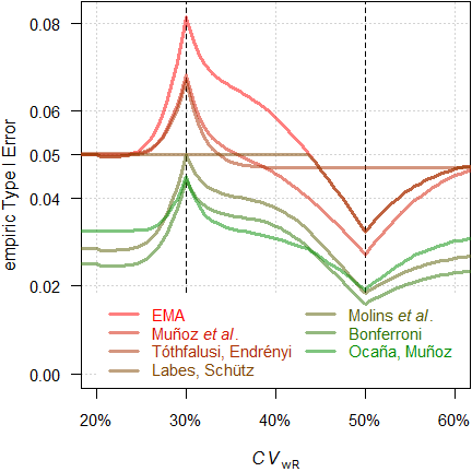
Fig. 18 Empiric TIE of
the approaches in a 4-period full replicate design (n 34).
We see an inflated Type I Error with the original ABEL in the critical region, as well as with the approaches of Muñoz et al.18 and Tóthfalusi and Endrényi.21 With all other approaches the TIE is controlled.
Power
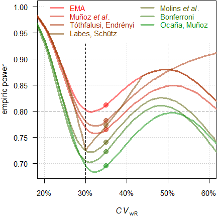
Fig. 19 Power of the approaches
in a 4-period full replicate design (n 34).
Filled circles
power for \(\small{CV_\textrm{wR}=CV_\textrm{wT}=35\%}\).
Since we planned for ABEL, we will achieve a power of 0.812 if the assumed \(\small{CV_\textrm{wR}}\) is realized in the study. With the approach of Tóthfalusi and Endrényi21 power will be 0.782, with the one of Labes and Schütz19 0.773, with the one of Muñoz _et al.18 0.765, with the one of Molins et al.22 0.740, with Bonferroni’s adjustment33 0.722, and with the approach of Ocaña and Muñoz24 0.695.
Ignoring the inflated Type I Error in some of the approaches: Which sample sizes would we need to maintain our target power and which sample size penalty compared to the original ABEL will we have to accept?
CV   <- 0.35
comp <- data.frame(method = rep(c("EMA (2010)",
                                  "Bonferroni (1936)",
                                  "Muñoz et al (2016)",
                                  "Labes and Schütz (2016)",
                                  "Molins et al. (2017)",
                                  "Tóthfalusi and Endrényi (2017)",
                                  "Ocaña and Muñoz (2019)"),
                                  each = length(CV)),
                   alpha = 0.05, n = NA_integer_, power = NA_real_)
for (i in 1:nrow(comp)) {
  if (comp$method[i] == "EMA (2010)") {
    comp[i, 3:4] <- sampleN.scABEL(CV = CV,
                                   design = "2x2x4",
                                   details = FALSE,
                                   print = FALSE)[8:9]
  }
  if (comp$method[i] == "Bonferroni (1936)") {
    comp[i, 2]   <- 0.025
    comp[i, 3:4] <- sampleN.scABEL(alpha = 0.025,
                                   CV = CV,
                                   design = "2x2x4",
                                   details = FALSE,
                                   print = FALSE)[8:9]
  }
  if (comp$method[i] == "Muñoz et al (2016)") {
    comp[i, 3:4] <- sampleN.RSABE(CV = CV,
                                  design = "2x2x4",
                                  regulator = "EMA",
                                  details = FALSE,
                                  print = FALSE)[8:9]
  }
  if (comp$method[i] == "Labes and Schütz (2016)") {
    res          <- sampleN.scABEL.ad(CV = CV,
                                      design = "2x2x4",
                                      details = FALSE,
                                      print = FALSE)
    comp[i, 2]   <- res$alpha.adj
    comp[i, 3:4] <- res[c(12, 14)]
  }
  if (comp$method[i] == "Molins et al. (2017)") {
    res        <- scABEL.ad(CV = 0.30, n = comp[1, 3],
                            design = "2x2x4",
                            details = FALSE,
                            print = FALSE)
    comp[i, 2] <- res$alpha.adj
    comp[i, 3] <- sampleN.scABEL.ad(alpha.pre = res$alpha.adj,
                                    CV = CV,
                                    design = "2x2x4",
                                    details = FALSE,
                                    print = FALSE)[["Sample size"]]
    comp[i, 4] <- power.scABEL(alpha = res$alpha.adj,
                               CV = CV, n = comp[i, 3],
                               design = "2x2x4")
  }
  if (comp$method[i] == "Tóthfalusi and Endrényi (2017)") {
    reg           <- reg_const("EMA")
    reg$CVcap     <- Inf
    reg$pe_constr <- FALSE
    reg$name      <- "pure EMA"
    comp[i, 3:4]  <- sampleN.RSABE2L.sds(CV = CV,
                                         design = "2x2x4",
                                         regulator = reg,
                                         details = FALSE,
                                         print = FALSE)[8:9]
  }
  if (comp$method[i] == "Ocaña and Muñoz (2019)") {
    if (adjustalpha.avail) {
      comp[i, 2] <- adjAlpha(n = comp[1, 3], beMethod = "HoweEMA",
                             design =  "TRTR-RTRT", nsim = 1e6,
                             seed = 123456)
  }else {
      comp[i, 2] <- 0.03225796 # hard-coded
    }
    res        <- sampleN.RSABE(alpha = comp[i, 2],
                                CV = CV, design = "2x2x4",
                                regulator = "EMA",
                                details = FALSE,
                                print = FALSE)
    comp[i, 3] <- res[["Sample size"]]
    comp[i, 4] <- res[["Achieved power"]]
  }
}
comp$alpha   <- round(comp$alpha, 5)
comp$power   <- signif(comp$power, 4)
comp$penalty <- sprintf("%+.1f%%", 100 * (comp$n - comp$n[1]) / comp$n[1])
comp$penalty[1] <- "   –"
print(comp, row.names = FALSE, right = FALSE)
# method alpha n power penalty
# EMA (2010) 0.05000 34 0.8118 –
# Bonferroni (1936) 0.02500 42 0.8035 +23.5%
# Muñoz et al (2016) 0.05000 38 0.8055 +11.8%
# Labes and Schütz (2016) 0.03610 38 0.8100 +11.8%
# Molins et al. (2017) 0.02857 40 0.8018 +17.6%
# Tóthfalusi and Endrényi (2017) 0.05000 38 0.8178 +11.8%
# Ocaña and Muñoz (2019) 0.03226 46 0.8128 +35.3%Conclusion‽
If the drug / drug product is not highly variable (\(\small{\sigma_\text{wR}<0.294}\)), the FDA’s RSABE and the GCC’s widened limits based on the observed \(\small{s_\text{wR}}\) lead to an extremely inflated Type I Error. Assessing the TIE with the ‘desired consumer risk model’28 29 is questionable.26 While adjusting \(\small{\alpha}\) is possible,1 2 3 likely the sample size penalty would be prohibitive in practice.
When it comes to
ABEL,
at least the approach of Labes and Schütz19 should be considered. However, it relies on
the plug-in
principle, i.e., assumes that the observed \(\small{CV_\text{wR}}\) is the true one.
Only if an inflated Type I Error is likely, it requires larger sample
sizes than the original
ABEL.
The approach of Molins et al.22
does not need this assumption and controls the Type I Error irrespective
of the observed \(\small{CV_\text{wR}}\). However, due to its
conservatism it requires larger sample sizes to maintain the target
power.
For an agency there are no reasons to object employing an
apparently more conservative \(\small{\alpha}\) in both approaches, as
evaluation with a 90% CI (\(\small{\alpha=0.05}\)) is a recommendation
and an applicant free to evaluate a study with a wider
CI (\(\small{\alpha<0.05}\)).26 39
The approach of Ocaña and Muñoz24
controls the TIE as well but requires a modification of the
statistical model stated in regulatory guidelines currently recommending
ABEL.
In most cases the impact on power is substantial (i.e., the
sample size has to be even larger than for Bonferroni’s
adjustment33).
While abandoning the upper cap of scaling in the approach of Tóthfalusi
and Endrényi21 might be possible (note
that there is none in the
FDA’s
RSABE and
the GCC’s widened limits
as well), dropping the PE-constraint
is somewhat utopian.
Acknowledgment
Jordi
Ocaña Rebull (Department of Genetics, Microbiology and Statistics,
Universitat de Barcelona, Spain), Eduard Molins
Lleonart (Universitat Politècnica de Catalunya, Spain), and Joel
Muñoz Gutiérrez (Faculty of Physical and Mathematical Sciences,
Department of Statistics, Universidad de Concepción, Chile) for fruitful
discussions and providing the packages simcrossover and
adjustalpha.
Licenses
 Helmut Schütz 2022
R, PowerTOST,
simcrossover, and adjustalpha GPL 3.0,
klippy MIT,
pandoc GPL 2.0.
1st version May 4, 2021. Rendered December 11, 2022 13:52 CET
by rmarkdown
via pandoc in 1.06 seconds.
Footnotes and References
Labes D, Schütz H, Lang B. PowerTOST: Power and Sample Size for (Bio)Equivalence Studies. Package version 1.5.4.9000. 2022-04-25. CRAN↩︎
Ocaña J. simcrossover: Data Generation from a Crossover Design as a data.frame. Package version 0.2.0. 2018-05-26.↩︎
Ocaña J. adjustalpha: Significance level adjustment in Scaled Average Bioequivalence. Package version 0.9.0. 2018-10-02.↩︎
Benet L. Bioequivalence of Highly Variable (HV) Drugs: Clinical Implications. Why HV Drugs are Safer. Presentation at: FDA Advisory Committee for Pharmaceutical Science. Rockville. 14 April, 2004.
 Internet
Archive.↩︎
Internet
Archive.↩︎Blume H, Mutschler E, editors. Bioäquivalenz. Qualitätsbewertung wirkstoffgleicher Fertigarzneimittel. Frankfurt/Main: Govi-Verlag; 6. Ergänzungslieferung 1996. [German].↩︎
Commission of the EC. Note for Guidance. Investigation of Bioavailability and Bioequivalence. Appendix III: Technical Aspects of Bioequivalence Statistics. Brussels. December 1991.↩︎
Commission of the EC. Note for Guidance. Investigation of Bioavailability and Bioequivalence. Appendix III: Technical Aspects of Bioequivalence Statistics. 3CC15a. Brussels. June 1992. Online.↩︎
EMA, CHMP Efficacy Working Party, Therapeutic Subgroup on Pharmacokinetics (EWP-PK). Questions & Answers on the Bioavailability and Bioequivalence Guideline. London. 27 July 2006. Online.↩︎
Benet L. Why Highly Variable Drugs are Safer. Presentation at the FDA Advisory Committee for Pharmaceutical Science. Rockville. 06 October, 2006.
Internet
Archive.↩︎Schütz H. ABEL: Type I Error. Vienna: Bioequivalence and Bioavailability Forum; 28 September 2020.↩︎
EMA. Clinical pharmacology and pharmacokinetics: questions and answers. 3.1 Which statistical method for the analysis of a bioequivalence study does the Agency recommend? Annex I. London. 21 September 2016. Online.↩︎
Zheng C, Wang J, Zhao L. Testing bioequivalence for multiple formulations with power and sample size calculations. Pharm Stat. 2012; 11(4): 334–41. doi:10.1002/pst.1522.↩︎
Tóthfalusi L, Endrényi L, García-Arieta A. Evaluation of bioequivalence for highly variable drugs with scaled average bioequivalence. Clin Pharmacokinet. 2009; 48(11): 725–43. doi:10.2165/11318040-000000000-00000.↩︎
Haidar SH, Makhlouf F, Schuirmann DJ, Hyslop T, Davit B, Conner D, Yu LX. Evaluation of a Scaling Approach for the Bioequivalence of Highly Variable Drugs. AAPS J. 2008; 10(3): 450–4. doi:10.1208/s12248-008-9053-4.
 Free
Full Text.↩︎
Free
Full Text.↩︎Endrényi L, Tóthfalusi L. Regulatory and Study Conditions for the Determination of Bioequivalence of Highly Variable Drugs. J Pharm Pharmaceut Sci. 2009; 12(1): 138–49. doi:10.18433/J3ZW2C.
 Open
Access.↩︎
Open
Access.↩︎Karalis V, Symillides M, Macheras P. On the leveling-off properties of the new bioequivalence limits for highly variable drugs of the EMA guideline. Europ J Pharm Sci. 2011; 44: 497–505. doi:10.1016/j.ejps.2011.09.008.↩︎
Wonnemann M, Frömke C, Koch A. Inflation of the Type I Error: Investigations on Regulatory Recommendations for Bioequivalence of Highly Variable Drugs. Pharm Res. 2015; 32(1): 135–43. doi:10.1007/s11095-014-1450-z.↩︎
Muñoz J, Alcaide D, Ocaña J. Consumer’s risk in the EMA and FDA regulatory approaches for bioequivalence in highly variable drugs. Stat Med. 2016; 35(12): 1933–43. doi:10.1002/sim.6834.↩︎
Labes D, Schütz H. Inflation of Type I Error in the Evaluation of Scaled Average Bioequivalence, and a Method for its Control. Pharm Res. 2016; 33(11): 2805–14. doi:10.1007/s11095-016-2006-1.↩︎
Tóthfalusi L, Endrényi L. An Exact Procedure for the Evaluation of Reference-Scaled Average Bioequivalence. AAPS J. 2016; 18(2): 476–89. doi:10.1208/s12248-016-9873-6.
Free
Full Text.↩︎Tóthfalusi L, Endrényi L. Algorithms for Evaluating Reference Scaled Average Bioequivalence: Power, Bias, and Consumer Risk. Stat Med. 2017; 36(27): 4378–90. doi:10.1002/sim.7440.↩︎
Molins E, Cobo E, Ocaña J. Two-Stage Designs Versus European Scaled Average Designs in Bioequivalence Studies for Highly Variable Drugs: Which to Choose? Stat Med. 2017; 36(30): 4777–88. doi:10.1002/sim.7452.↩︎
Endrényi L, Tóthfalusi L. Bioequivalence for highly variable drugs: regulatory agreements, disagreements, and harmonization. J Pharmacokin Pharmacodyn. 2019; 46(2): 117–26. doi:10.1007/s10928-019-09623-w.↩︎
Ocaña J, Muñoz J. Controlling type I error in the reference-scaled bioequivalence evaluation of highly variable drugs. Pharm Stat. 2019; 18(5): 583–99. doi:10.1002/pst.1950.↩︎
Deng Y, Zhou X-H. Methods to control the empirical type I error rate in average bioequivalence tests for highly variable drugs. Stat Methods Med Res. 2019; 29(6): 1650–67. doi:10.1177/0962280219871589.↩︎
Schütz H, Labes D, Wolfsegger MJ. Critical Remarks on Reference-Scaled Average Bioequivalence. J Pharm Pharmaceut Sci. 25: 285–96. doi:10.18433/jpps32892.↩︎
Berger RL, Hsu JC. Bioequivalence Trials, Intersection–Union Tests and Equivalence Confidence Sets. Stat Sci. 1996; 11(4): 283–319. doi:10.1214/ss/1032280304.↩︎
Davit BM, Chen ML, Conner DP, Haidar SH, Kim S, Lee CH, Lionberger RA, Makhlouf FT, Nwakama PE, Patel DT, Schuirmann DJ, Yu LX. Implementation of a Reference-Scaled Average Bioequivalence Approach for Highly Variable Generic Drug Products by the US Food and Drug Administration. AAPS J. 2012; 14(4): 915–24. doi:10.1208/s12248-012-9406-x.
Free
Full Text.↩︎Schuirmann DJ. U. S. FDA Perspective: Statistical Aspects of OGD’s Approach to Bioequivalence (BE) Assessment for Highly Variable Drugs. Presentation at: The Global Bioequivalence Harmonization Initiative: EUFEPS/AAPS Second International Conference. Rockville. September 15–16, 2016.↩︎
FDA, OGD. Draft Guidance on Progesterone. Rockville. Recommended April 2010, Revised February 2011. Download.↩︎
FDA, CDER. Bioequivalence Studies With Pharmacokinetic Endpoints for Drugs Submitted Under an ANDA. Silver Spring. August 2021. Download.↩︎
Detlew Labes and László Endrényi, just to name some.↩︎
Bonferroni CE. Teoria statistica delle classi e calcolo delle probabilità. Pubbl. R Ist. Sup. Sci. Econ. Commer. Fir. 1936. 8; 1–62. [Italian].↩︎
Howe WG. Approximate Confidence Limits on the Mean of X + Y Where X and Y Are Two Tabled Independent Random Variables. J Am Stat Assoc. 1974; 69: 789–94. doi:10.2307/2286019.↩︎
Hedges LV. Distribution Theory for Glass’s Estimator of Effect Size and Related Estimators. J Educ Stat. 1981; 6(2): 107–28. doi:10.2307/1164588.↩︎
The authors may forgive me using quotation marks. Hedges’ correction is an approximation.↩︎
Sun W. Re-cap from last meeting and new evidence comparing EMA, HC, FDA approach for highly variable drugs and replicate design; consumer risk? Presentation at: The Global Bioequivalence Harmonisation Initiative: EUFEPS/AAPS Fifth International Conference. Amsterdam. 28–29 September 2022.↩︎
Schütz H. Consumer risk in SABE. Contribution to the discussion at: The Global Bioequivalence Harmonisation Initiative: EUFEPS/AAPS Fifth International Conference. Amsterdam. 28–29 September 2022. Online.↩︎
• Junior (read naïve) assessor
I don’t have the slightest clue why the applicant used a wider CI, which increases the chance of failure because power will by lower than with a 90% CI. It’s not my job to by concerned about the producer’s risk (I was told that post hoc power does not play any role in BE). Since the study passed with a wider CI, MA granted.
• Senior (hopefully expert) assessor
Seemingly the applicant is concerned about the consumer risk and it is controlled with the method, which was stated in the protocol. Since the study passed with a wider CI, MA granted.
• Both
Naturally, the study would have passed with the 90% CI as recommended in the guideline as well. Fine with me.↩︎