Preliminaries

A basic knowledge of R does not hurt. To run the scripts at least version 1.2-1 (2014-09-30) of PowerTOST is required and for the GCC’s approach at least version 1.5-3 (2021-01-18). Any version of R would likely do, though the current release of PowerTOST was only tested with version 4.1.3 (2022-03-10) and later. All scripts were run on a Xeon E3-1245v3 @ 3.40GHz (1/4 cores) 16GB RAM with R 4.2.0 on Win­dows 7 build 7601, Service Pack 1, Universal C Runtime 10.0.10240.16390.

Note that in all functions of PowerTOST the arguments (say, the assumed T/R-ratio theta0, the BE-limits (theta1, theta2), the assumed coefficient of variation CV, etc.) have to be given as ratios and not in percent.

Sample sizes are given for equally sized groups (parallel design) and for balanced sequences (crossovers, replicate designs). Furthermore, the estimated sample size is the total number of subjects, which is always an even number (parallel design) or a multiple of the number of sequence (crossovers, replicate designs) – not subjects per group or sequence like in some other software packages.

top of section ↩︎ previous section ↩︎

Terminology

In order to get prospective power (and hence, a sample size), we need five values:

1. The level of the test \(\small{\alpha}\) (in BE commonly 0.05),
2. the BE-margins (commonly 0.80 – 1.25),
3. the desired (or target) power \(\small{\pi}\),
4. the variance (commonly expressed as a coefficient of variation), and
5. the deviation of the test from the reference treatment.

1 – 2 are fixed by the agency,
3 is set by the sponsor (commonly to 0.80 – 0.90), and
4 – 5 are just (uncertain!) assumptions.

Since it is extremely unlikely that all assumptions will be exactly realized in a particular study, it is worthwhile to prospectively explore the impact of potential deviations from assumptions on power.

We don’t have to be concerned about values which are ‘better’ (i.e., a lower CV, and/or a T/R-ratio closer to unity, and/or a lower than anticipated dropout-rate) because we will gain power. On the other hand, any change towards the ‘worse’ will negatively impact power.

top of section ↩︎ previous section ↩︎

Parallel Design

We assume a CV of 0.40, a T/R-ratio of 0.95, target a power of 0.80 (see also the example in the corresponding article about the parallel design), and keep the default minimum power 0.70.

CV <- 0.40
x  <- pa.ABE(CV = CV, design = "parallel") # assign to an object
dev.new(width = 6.2, height = 6.7)
op <- par(no.readonly = TRUE)
plot(x, pct = FALSE, ratiolabel = "theta0")
par(op)
print(x, plot.it = FALSE)

# Sample size plan ABE
#    Design alpha  CV theta0 theta1 theta2 Sample size
#  parallel  0.05 0.4   0.95    0.8   1.25         130
#  Achieved power
#        0.803512
# 
# Power analysis
# CV, theta0 and number of subjects leading to min. acceptable power of ~0.7:
#  CV= 0.4552, theta0= 0.9276
#  n = 103 (power= 0.701)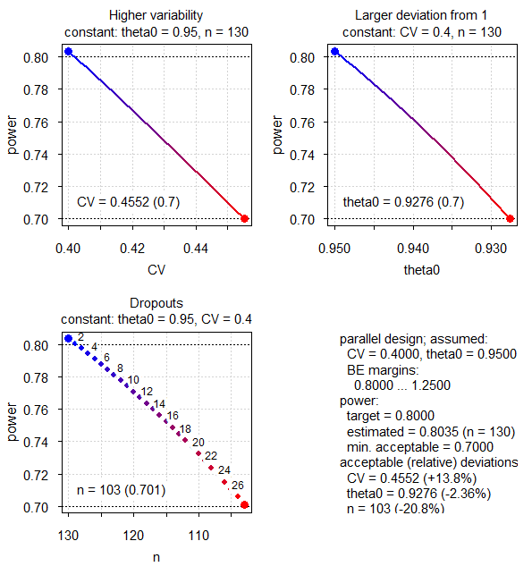

Fig.1 Parallel design (CV 0.40, T/R ratio 0.95).

Such patterns are typical for ABE. Note that the x-axes of the second and third panels are reversed (decreasing).

The most sensitive parameter is the T/R-ratio \(\small{\theta_0}\), which can decrease from the assumed 0.95 to 0.9276 (maximum relative deviation –2.36%) until we reach our minimum acceptable power of 0.70. The CV is much less sensitive, which can increase from the assumed 0.40 to 0.4552 (relative +13.8%). The least sensitive is the sample size itself, which can decrease from the planned 130 subjects to 103 (relative –20.8%). Hence, dropouts are in general of the least concern.

top of section ↩︎ previous section ↩︎

Crossover Design

Conventional ABE

We assume a CV of 0.25, a T/R-ratio of 0.95, target a power of 0.80 (see also the example in the corresponding article about the 2×2×2 design), and keep the default minimum power 0.70.

CV <- 0.25
x  <- pa.ABE(CV = CV)
dev.new(width = 6.2, height = 6.7)
op <- par(no.readonly = TRUE)
plot(x, pct = FALSE, ratiolabel = "theta0")
par(op)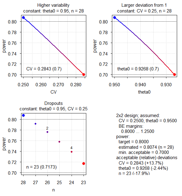

Fig.2 2×2×2 design (CV 0.25, T/R ratio 0.95).

The order of parameters influencing power is as common in ABE: \(\small{\theta_0}\) \(\small{\gg}\) CV \(\small{>}\) n.

top of section ↩︎ previous section ↩︎

ABE for NTIDs

We assume a CV of 0.125, a T/R-ratio of 0.975, target a power of 0.80 (see also the example in the corresponding article about the 2×2×2 design), and keep the default minimum power 0.70.

CV     <- 0.125
theta0 <- 0.975
theta1 <- 0.90
x  <- pa.ABE(CV = CV, theta0 = theta0, theta1 = theta1)
dev.new(width = 6.2, height = 6.7)
op <- par(no.readonly = TRUE)
plot(x, pct = FALSE, ratiolabel = "theta0")
par(op)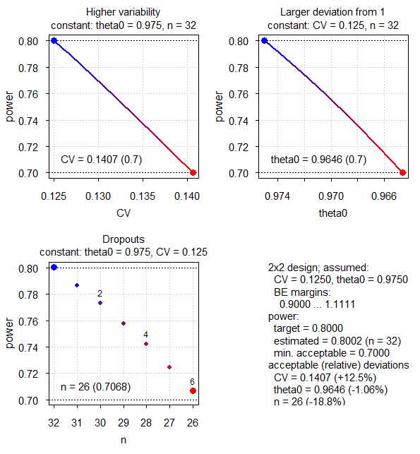

Fig.3 2×2×2 design (CV 0.125, T/R ratio 0.975, NTID).

Business as usual.

top of section ↩︎ previous section ↩︎

HVDs / HVDPs

ABEL

EMA and most others

We assume a CV of 0.45, a T/R-ratio of 0.90, target a power of 0.80 (see also the example in the corresponding article), keep the default minimum power 0.70, and want to perform the study in a 2-sequence 4-period full replicate study (TRTR|RTRT or TRRT|RTTR or TTRR|RRTT).

CV     <- 0.45
design <- "2x2x4"
x      <- pa.scABE(CV = CV, design = design)
dev.new(width = 6.2, height = 6.7)
op      <- par(no.readonly = TRUE)
plot(x, pct = FALSE, ratiolabel = "theta0")
par(op)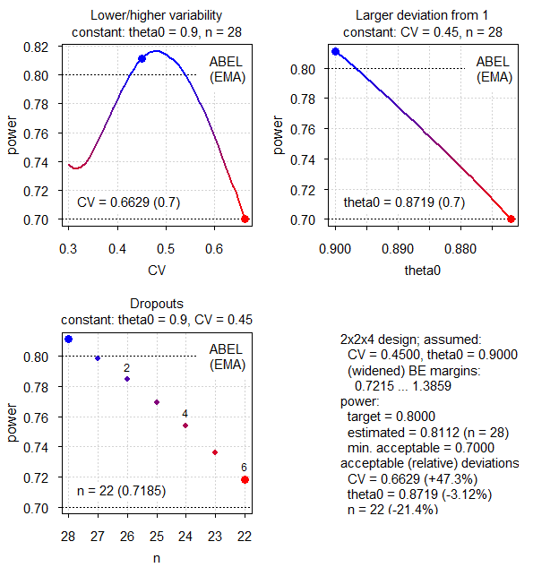

Fig.3 2×2×4 replicate design (CV 0.45, T/R ratio 0.90, ABEL for the EMA).

Here the pattern is different to ABE. The idea of reference-scaling is to maintain power irrespective of the CV. Therefore, the CV is the least sensitive parameter – it can increase from the assumed 0.45 to 0.6629 (relative +47.3%). If the CV decreases, power decreases as well because we can expand limits less.

    

Let’s dive deeper. x is an S3 object.¹¹ Contained in its list are the data.frames paCV, paGMR, and paN. With the function power.scABEL() we can assess the components of power at specific values of the CV.

n       <- x$paN$N[1]
max.pwr <- which(x$paCV$pwr == max(x$paCV$pwr))
CVs     <- c(head(x$paCV$CV, 1),
             x$paCV$CV[x$paCV$pwr == min(x$paCV$pwr[1:max.pwr])],
             CV, x$paCV$CV[max.pwr], tail(x$paCV$CV, 1))
res     <- data.frame(CV = CVs, V1 = NA, V2 = NA, V3 = NA, V4 = NA)
for (i in 1:nrow(res)) {
  res[i, 2:5] <- suppressMessages(
                   power.scABEL(CV = CVs[i], design = design,
                                n = n, details = TRUE))
}
names(res)[2:5] <- c("p(BE)", "p(BE-ABEL)",
                     "p(BE-PE)", "p(BE-ABE)")
print(signif(res, 4), row.names = FALSE)

#      CV  p(BE) p(BE-ABEL) p(BE-PE) p(BE-ABE)
#  0.3000 0.7383     0.7383   0.9832    0.6786
#  0.3167 0.7351     0.7351   0.9784    0.6403
#  0.4500 0.8112     0.8116   0.9266    0.4107
#  0.4766 0.8164     0.8165   0.9161    0.3764
#  0.6629 0.7000     0.7000   0.8467    0.1546

p(BE) is the overall power, p(BE-ABEL) is the power of ‘pure’ ABEL (without the PE-restriction), and p(BE-PE) is the power of the criterion ‘point estimate within acceptance range’ alone. p(BE-ABE) is the power of the conventional ABE test for comparative purposes.

We see that close to the upper cap of scaling (at CV 50%) power starts to decrease because we cannot expand the limits any more (maximum expansion 69.84 – 143-19%). Furthermore, the PE-restriction becomes increasingly important.

top of section ↩︎ previous section ↩︎

Health Canada

As above but according to the rules of Health Canada (upper cap of scaling ~57.4% instead of 50%).¹²

CV     <- 0.45
design <- "2x2x4"
x      <- pa.scABE(CV = CV, design = design,
                   regulator = "HC")
dev.new(width = 6.2, height = 6.7)
op      <- par(no.readonly = TRUE)
plot(x, pct = FALSE, ratiolabel = "theta0")
par(op)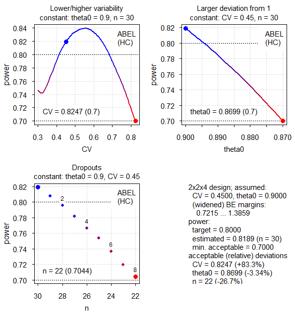

Fig.4 2×2×4 replicate design (CV 0.45, T/R ratio 0.90, ABEL for Health Canada).

Similar to the EMA but more relaxed due to the higher upper cap.

top of section ↩︎ previous section ↩︎

GCC

That’s a special case because for any CV > 30% the limits are directly widened to 75.00 – 133.33% and there is no upper cap of scaling.¹³

CV     <- 0.45 # at least v1.5.3 of PowerTOST required
design <- "2x2x4"
x      <- pa.scABE(CV = CV, design = design,
                   regulator = "GCC")
dev.new(width = 6.2, height = 6.7)
op      <- par(no.readonly = TRUE)
plot(x, pct = FALSE, ratiolabel = "theta0")
par(op)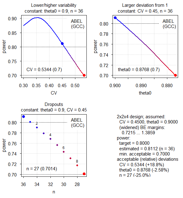

Fig.5 2×2×4 replicate design (CV 0.45, T/R ratio 0.90, ABEL for the GCC).

top of section ↩︎ previous section ↩︎

RSABE

As above but for the U.S. FDA and China’s CDE (see also the example in the corresponding article).

CV     <- 0.45
design <- "2x2x4"
x      <- pa.scABE(CV = CV, design = design,
                   regulator = "FDA")
dev.new(width = 6.2, height = 6.7)
op      <- par(no.readonly = TRUE)
plot(x, pct = FALSE, ratiolabel = "theta0")
par(op)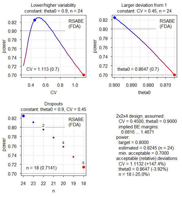

Fig.6 2×2×4 replicate design (CV 0.45, T/R ratio 0.90, RSABE).

Due to unlimited scaling the CV is even less important than in the other methods.

top of section ↩︎ previous section ↩︎

NTIDs

We assume a CV of 0.125, a T/R-ratio of 0.975 (the function’s default), target a power of 0.80, and want to perform the study in a 2-sequence 4-period full replicate study (TRTR|RTRT or TRRT|RTTR or TTRR|RRTT). Note that such a design is mandatory for the FDA and China’s CDE. See also the example in the corresponding article.

CV     <- 0.125
design <- "2x2x4"
x      <- pa.NTID(CV = CV, design = design)
dev.new(width = 6.2, height = 6.9)
op      <- par(no.readonly = TRUE)
plot(x, pct = FALSE, ratiolabel = "theta0")
par(op)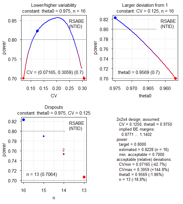

Fig.7 2×2×4 replicate design (CV 0.125, T/R ratio 0.975, RSABE for NTIDs).

Here the CV shows a different behavior to both RSABE for HVDs / HVDPs and ABE (see above). Maximum power is seen at ~20.4% and we observe two minima.

top of section ↩︎ previous section ↩︎