Consider allowing JavaScript. Otherwise, you have to be proficient in reading LaTeX since formulas will not be rendered. Furthermore, the table of contents in the left column for navigation will not be available and code-folding not supported. Sorry for the inconvenience.

Examples in this article were generated with 4.2.1 by the package PowerTOST.¹

Click to show / hide R code.
Click on the icon in the top left corner to copy R code to the clipboard .

Introduction

Why may we need a Power Table?

Convenience. Of course, you could write your own script (calculating power while looping over sample sizes). However, it would require adaption for the many methods implemented in PowerTOST. This article was inspired by a post at the BEBA-Forum.²

In the sample size functions of PowerTOST with the argument details = TRUE we get only the final steps of the sample size search. In the functions for power analysis (pa.ABE, pa.scABE, pa.NTID), we can specify a minimum acceptable power but not adjust for an anticipated dropout-rate. Furthermore, heteroscedasticity (CV_wT ≠ CV_wR) is not supported and we would have to read power dependent on the sample size from a figure.

Preliminaries

A basic knowledge of R does not hurt. To run the scripts at least version 1.2-1 (2014-09-30) of PowerTOST is required and for the GCC’s approach at least version 1.5-3 (2021-01-18). Any version of R would likely do, though the current release of PowerTOST was only tested with version 4.1.3 (2022-03-10) and later. All scripts were run on a Xeon E3-1245v3 @ 3.40GHz (1/4 cores) 16GB RAM with R 4.2.1 on Windows 7 build 7601, Service Pack 1, Universal C Runtime 10.0.10240.16390.

Note that in all functions of PowerTOST the arguments (say, the assumed T/R-ratio theta0, the BE-margins (theta1, theta2), the assumed coefficient of variation CV, etc.) have to be given as ratios and not in percent. Only fixed-sample designs for equivalence (single site, single group) are covered.

Sample sizes are estimated for equally sized groups (parallel design) and for balanced sequences (crossovers, replicate designs). Furthermore, the estimated sample size is the total number of subjects, which is always an even number (parallel design) or a multiple of the number of sequence (crossovers, replicate designs) – not subjects per group or sequence like in some other software packages.

top of section ↩︎ previous section ↩︎

R Script

The function power.table() supports all designs applicable for a given method. The defaults are:

Argument	Default	Meaning
`ABE`	`TRUE`	Assess for Average Bioequivalence (ABE). Set to `FALSE` for Scaled Average Bioequivalence (SABE) by Reference-Scaled Average Bioequivalence (RSABE) or Average Bioequivalence with Expanding Limits (ABEL).
`alpha`	`0.05`	Nominal level of the test \(\small{\alpha}\), probability of the Type I Error (patient’s risk)
`bal`	`TRUE`	Gives equally sized groups (parallel design) or balanced sequences (crossover and replicate designs)
`design`	→	`"2x2x2"` if `ABE = TRUE` `"2x3x3"` if `ABE = FALSE` `"2x2x4"` if `NTID = TRUE`
`do.rate`	`0`	Anticipated dropout-rate. If > 0 adjusts the sample size accordingly.
`method`	`"exact"`	Observed only if `ABE = TRUE`. Power estimation method; alternatives are `"nct"` for the noncentral t-distribution and `"shifted"` for the shifted central t-distribution.
`minpower`	`0.70`	Minimum acceptable power
`nsims`	`1e5`	Observed only if `ABE = FALSE` or `NTID = TRUE`; number of simulations in SABE
`NTID`	`FALSE`	If `TRUE`, assess a Narrow Theraputic Index Drug (NTID) by RSABE
`print`	`TRUE`	If `TRUE` (default), results are printed to the console
`regulator`	`"EMA"`	Observed only if `ABE = FALSE`; implemented are `"EMA"` (European Medicines Agency and others), `"HC"` (Health Canada), `"GCC"` (Gulf Cooperation Council), and `"FDA"` (U.S. Food and Drug Administration, China’s Center for Drug Evaluation)
`targetpower`	`0.80`	Target (desired) power \(\small{\pi = 1-\beta}\), where \(\small{\beta}\) is the probability of the Type II Error (producer’s risk)
`theta0`	→	Assumed T/R-ratio `0.95` if `ABE = TRUE` `0.90` if `ABE = FALSE` `0.975` if `NTID = TRUE` or `ABE = TRUE` and `theta1 = 0.90`
`theta1`	`0.80`	Lower BE-margin in ABE and lower PE-constraint in SABE
`theta2`	`1.25`	Upper BE-margin in ABE and upper PE-constraint in SABE
`TIE`	`FALSE`	If `TRUE`, assess the empiric Type I Error of SABE in 10⁶ simulations

When specifying CV as a two-element vector in SABE, the first element has to be the within-subject CV of the test product (CV_wT) and the second the one of the reference (CV_wR).

I suggest to save the script (any file name with the extension R would do). Then you can source it in the R-console or an IDE like RStudio and call the function power.table() with suitable arguments. Generally a one-liner.

Terribly sorry, 604 (‼) LOC. Flexibility comes with a price.

power.table <- function(alpha = 0.05, CV = CV, theta0, theta1, theta2,
                        design, ABE = TRUE, method = "exact", NTID = FALSE,
                        target = 0.8, minpower = 0.7, bal = TRUE, do.rate = 0,
                        regulator = "EMA", nsims = 1e5, TIE = FALSE,
                        details = TRUE) {
  ###########################################################################
  # Arguments:                                                              #
  # alpha    : Nominal level of the test (default 0.05)                     #
  # CV       : within-subject (crossovers, paired design), total (parallel) #
  #            can be a two-element vector for SABE; first element CVw of T #
  #            and second element CVw of R                                  #
  # theta0   : assumed T/R-ratio (default 0.95 for ABE, 0.90 for SABE,      #
  #            0.975 for NTID and ABE if theta1 = 0.9 or theta1 = 1 / 0.9   #
  # theta1   : lower BE-limit (ABE/NTID), lower PE-constraint (SABE)        #
  #            default 0.80 for ABE/NTID, fixed PE-constraint 0.80 for SABE #
  # theta2   : upper BE-limit (ABE/NTID), upper PE-constraint (SABE)        #
  #            default 1.25 for ABE/NTID, fixed PE-constraint 1.25 for SABE #
  # design   : any supported; see known.designs()                           #
  #            defaults: "2x2x2" for ABE, "2x3x3" for SABE (ABEL and RSABE) #
  #                      "2x2x4" for NTIDs                                  #
  # ABE      : TRUE (default) for ABE, FALSE for SABE                       #
  # method   : ABE only; power method (default "exact")                     #
  # NTID     : FALSE (default), TRUE for RSABE (FDA, CDE)                   #
  # target   : target (desired) power (default 0.8)                         #
  # minpower : minimum acceptable power (default 0.7)                       #
  #            analog to pa.ABE(), pa.scABE(), pa.NTID()                    #
  # do.rate  : anticipated dropout rate (default 0); if > 0, the estimated  #
  #            sample size will be adjusted in order to have at least the   #
  #            estimated sample size in the worst case                      #
  # bal      : should only balanced sequences (crossovers, replicates) or   #
  #            equal group sizes (parallel) be shown (default TRUE)?        #
  # nsims    : SABE only; number of simulations for SABE (default 1e5)      #
  # regulator: SABE only; any of "EMA", "HC", "GCC", "FDA" (default "EMA")  #
  # TIE      : SABE only; empiric Type I Error (default FALSE)              #
  # details  : should the aggregated results and data frame be printed      #
  #            (default TRUE)?                                              #
  # ----------------------------------------------------------------------- #
  # Notes                                                                   #
  # - Only for the multiplicative model, i.e., in PowerTOST’s functions for #
  #   ABE logscale = TRUE is applied                                        #
  # - If simulating the empiric Type I Error 1e6 simulations are employed   #
  # - Sample size adjustments are tricky; I hope to have covered them       #
  #   correctly:                                                            #
  #   - In general 12 _eligible_ subjects are required                      #
  #   - The EMA requires for ABEL 12 _eligible_ subjects in a 2-sequence 3- #
  #     period full replicate design in the RR-sequence, i.e., 24 total     #
  #   - In RSABE (FDA and CDE) we need 24 _dosed_ subjects                  #
  #   - there is no minimum sample size for RSABE of NTIDS given in the     #
  #     guidance; I assumed 12 _eligible_ subjects                          #
  ###########################################################################
  require(PowerTOST)
  balance <- function(n, n.seq) {
    # Round up the sample size to obatain equally sized sequences (crossover /
    # replicate designs) or groups (parallel design)
    return(as.integer(n.seq * (n %/% n.seq + as.logical(n %% n.seq))))
  }
  nadj <- function(n, do.rate, n.seq) {
    # Adjust the sample size for the anticipated dropout-rate
    return(as.integer(balance(n / (1 - do.rate), n.seq)))
  }
  # Input checking: Error handling, dealing with missing arguments,
  #                 messages about strange input
  CV <- abs(CV)
  if (NTID) ABE <- FALSE # we apply RSABE
  if (ABE & length(CV) > 1)
    stop("Give \"CV\" as a one element vector for ABE.")
  if (!ABE & length(CV) > 2)
    stop("\"CV\" must have not more than two elements for SABE.")
  if (!ABE & !regulator %in% c("EMA", "FDA", "HC", "GCC"))
    stop("regulator \"", regulator, "\" not supported.")
  if (missing(design)) {
    if (ABE)          design <- "2x2x2"
    if (!ABE & !NTID) design <- "2x3x3"
    if (NTID)         design <- "2x2x4"
  }
  if (!ABE & !design %in% c("2x3x3", "2x2x4", "2x2x3"))
    stop("A replicate design is required for reference-scaling.")
  if (NTID & !design %in% c("2x2x4", "2x2x3"))
    stop("A full replicate design is required for reference-scaling.")
  if (missing(theta1) & missing(theta2)) theta1 <- 0.80
  if (missing(theta1)) theta1 <- 1/theta2
  if (missing(theta2)) theta2 <- 1/theta1
  if (!method %in% c("exact", "owenq", "mvt", "noncentral",
                     "nct", "central", "shifted"))
    stop("method \"", method, "\" not supported.")
  if (target <= 0.5) stop("\"target = ", target, "\" does not make sense.")
  if (minpower <= 0.5) stop("\"minpower = ", minpower,
                            "\" does not make sense.")
  if (minpower >= target) stop("\"minpower\" must be < \"target\".")
  if (nsims < 5e4) message("Note: sample size based on < 50,000",
                           "\n      simulations may be unreliable.")
  do.rate <- abs(do.rate)
  if (do.rate > 0 & do.rate >= 0.5) stop("\"do.rate = ", do.rate,
                                         "\" does not make sense.")
  if (NTID) {
    # Not a good idea to fiddle with the limits!
    if (!theta1 == 0.8) {
      message(sprintf("Note: theta1 = %.4f ", theta1),
                      "\n      not compliant with the guidance.")
    }
    if (!theta2 == 1.25) {
      message(sprintf("Note: theta2 = %.4f ", theta2),
                      "\n      not compliant with the guidance.")
    }
  }
  # Default theta0 for the various approaches
  if (missing(theta0)) {
    if (NTID | theta1 == 0.9 | theta2 == 1 / 0.9) {
      theta0 <- 0.975
  }else {
      ifelse (ABE, theta0 <- 0.95, theta0 <- 0.9)
    }
  }
  # End of input checking
  if (!ABE) {# for SABE and NTID
    if (length(CV) == 2) {
      CVwT <- CV[1]
      CVwR <- CV[2]
  }else {
      CVwT <- CVwR <- CV
    }
  }
  # Minimum sample sizes acc. to GLs
  if (ABE | NTID) {
    min.n <- 12                          # eligible
}else {
    if (regulator %in% c("HC", "GCC")) {
      min.n <- 12                        # eligible
  }else {
      if (regulator == "FDA") {
        min.n <- 24                      # dosed
    }else {# EMA
        if (!design == "2x2x3") {
          min.n <- 12                    # eligible
      }else {
          min.n <- 24                    # eligible
        }
      }
    }
  }
  adj     <- FALSE # default if no dropouts or sample size compliant with GLs
  designs <- known.designs()[, c(1:2, 5)]
  n.step  <- n.seq <- designs[designs$design == design, "steps"]
  if (!bal) n.step <- 1L
  if (NTID) {
    tmp <- sampleN.NTID(alpha = alpha, CV = CV, theta0 = theta0,
                        theta1 = theta1, theta2 = theta2, targetpower = target,
                        design = design, nsims = nsims, details = FALSE,
                        print = FALSE)
    n   <- n.orig <- tmp[["Sample size"]]
    pwr.orig      <- tmp[["Achieved power"]]
    if (n < min.n) {# 12; nothing in the guidance - or is it 24 like in RSABE?
      n   <- min.n
      adj <- TRUE
    }
    if (do.rate > 0) {
      n.est <- n
      n     <- nadj(n, do.rate, n.seq)
      adj   <- TRUE
    }
    n.lo <- sampleN.NTID(alpha = alpha, CV = CV, theta0 = theta0,
                         theta1 = theta1, theta2 = theta2,
                         targetpower = minpower, design = design, nsims = nsims,
                         details = FALSE, print = FALSE)[["Sample size"]]
}else {
    if (ABE) {
      tmp <- sampleN.TOST(alpha = alpha, CV = CV, theta0 = theta0,
                          theta1 = theta1, theta2 = theta2,
                          targetpower = target, design = design,
                          method = method, print = FALSE)
      n   <- n.orig <- tmp[["Sample size"]]
      pwr.orig      <- tmp[["Achieved power"]]
      if (n < min.n) {
        n   <- min.n
        adj <- TRUE
      }
      if (do.rate > 0) {
        n.est <- n
        n     <- nadj(n, do.rate, n.seq)
        adj   <- TRUE
      }
      if (bal) {
        n.lo <- sampleN.TOST(alpha = alpha, CV = CV, theta0 = theta0,
                             theta1 = theta1, theta2 = theta2,
                             targetpower = minpower, design = design,
                             method = method, print = FALSE)[["Sample size"]]
    }else {
        # this section lifted/adapted from PowerTOST / pa.ABE.R
        n.est <- n
        Ns    <- seq(n.est, 12)
        if (n.est == 12) Ns <- seq(n.est, 2 * n.step)
        nNs   <-length(Ns)
        pwrN  <- power.TOST(alpha = alpha, CV = CV, theta0 = theta0,
                            theta1 = theta1, theta2 = theta2,
                            design = design, method = method, n = n)
        n.min <- NULL
        pBEn  <- NULL
        n     <- numeric(n.step)
        ni    <- 1:n.step
        i     <- 0
        while (pwrN >= minpower & i < nNs) {
          i          <- i + 1
          n[-n.step] <- diff(floor(Ns[i] * ni / n.step))
          n[n.step]  <- Ns[i] - sum(n[-n.step])
          pwrN       <- suppressMessages(
                          power.TOST(alpha = alpha, CV = CV, theta0 = theta0,
                                     theta1 = theta1, theta2 = theta2,
                                     design = design, method = method, n = n))
          if (pwrN >= minpower) {
            n.min <- c(n.min, sum(n))
            pBEn <- c(pBEn, pwrN)
        }else {
            break
          }
        }
        n    <- max(n.min)
        n.lo <- min(n.min)
      }
  }else {
      if (regulator == "FDA") {
        tmp <- sampleN.RSABE(alpha = alpha, CV = CV, theta0 = theta0,
                             targetpower = target, design = design,
                             nsims = nsims, details = FALSE, print = FALSE)
        n   <- n.orig <- tmp[["Sample size"]]
        pwr.orig      <- tmp[["Achieved power"]]
        if (n < min.n) {
          n   <- min.n
          adj <- TRUE
        }
        if (do.rate > 0) {
          n.est <- n
          n     <- nadj(n, do.rate, n.seq)
          adj   <- TRUE
        }
        if (bal) {
          n.lo <- sampleN.RSABE(alpha = alpha, CV = CV, theta0 = theta0,
                                targetpower = minpower, design = design,
                                nsims = nsims, details = FALSE,
                                print = FALSE)[["Sample size"]]
      }else {
          # this section lifted/adapted from PowerTOST / pa.scABE.R
          n.est <- n
          Ns    <- seq(n.est, 12)
          if (n.est == 12) Ns <- seq(n.est, 2 * n.step)
          nNs   <-length(Ns)
          pwrN  <- power.RSABE(alpha = alpha, CV = CV, theta0 = theta0,
                               design = design, n = n, nsims = nsims)
          n.min <- NULL
          pBEn  <- NULL
          n     <- numeric(n.step)
          ni    <- 1:n.step
          i     <- 0
          while(pwrN >= minpower & i < nNs){
            i    <- i + 1
            pwrN <- suppressMessages(
                      power.RSABE(alpha = alpha, CV = CV, theta0 = theta0,
                                  design = design, n = Ns[i], nsims = nsims))
            if (pwrN >= minpower) {
              n.min <- c(n.min, Ns[i])
              pBEn  <- c(pBEn, pwrN)
          }else {
              break
            }
          }
          n    <- max(n.min)
          n.lo <- min(n.min)
        }
    }else {
        if (!regulator == "HC" & design == "2x3x3" & CVwT > CVwR) {
          # Subject simulations if partial replicate and heteroscedasticity,
          # where T is more variable than R
          cat("Patience please. Simulating subject data is time consuming.\n")
          flush.console()
          tmp <- sampleN.scABEL.sdsims(alpha = alpha, CV = CV, theta0 = theta0,
                                       targetpower = target, design = design,
                                       regulator = regulator, nsims = nsims,
                                       details = FALSE,
                                       print = FALSE)
          n   <- n.orig <- tmp[["Sample size"]]
          pwr.orig      <- tmp[["Achieved power"]]
          n.lo <- sampleN.scABEL.sdsims(alpha = alpha, CV = CV, theta0 = theta0,
                                       targetpower = minpower, design = design,
                                       regulator = regulator, nsims = nsims,
                                       details = FALSE,
                                       print = FALSE)[["Sample size"]]
      }else {
          tmp <- suppressWarnings(
                   sampleN.scABEL(alpha = alpha, CV = CV, theta0 = theta0,
                                  targetpower = target, design = design,
                                  regulator = regulator, nsims = nsims,
                                  details = FALSE,
                                  print = FALSE))
          n   <- n.orig <- tmp[["Sample size"]]
          pwr.orig      <- tmp[["Achieved power"]]
          if (n < min.n) {
            n   <- min.n
            adj <- TRUE
          }
          if (do.rate > 0) {
            n.est <- n
            n     <- nadj(n, do.rate, n.seq)
            adj   <- TRUE
          }
          if (bal) {
            n.lo <- sampleN.scABEL(alpha = alpha, CV = CV, theta0 = theta0,
                                   targetpower = minpower, design = design,
                                   regulator = regulator, nsims = nsims,
                                   details = FALSE,
                                   print = FALSE)[["Sample size"]]
        }else {
            # this section lifted/adapted from PowerTOST / pa.scABE.R
            n.est <- n
            Ns    <- seq(n.est, 12)
            if (n.est == 12) Ns <- seq(n.est, 2 * n.step)
            nNs   <-length(Ns)
            pwrN  <- power.scABEL(alpha = alpha, CV = CV, theta0 = theta0,
                                 design = design, regulator = regulator, n = n,
                                 nsims = nsims)
            n.min <- NULL
            pBEn  <- NULL
            n     <- numeric(n.step)
            ni    <- 1:n.step
            i     <- 0
            while(pwrN >= minpower & i < nNs){
              i    <- i + 1
              pwrN <- suppressMessages(
                        power.scABEL(alpha = alpha, CV = CV, theta0 = theta0,
                                    design = design, regulator = regulator,
                                    n = Ns[i], nsims = nsims))
              if (pwrN >= minpower) {
                n.min <- c(n.min, Ns[i])
                pBEn  <- c(pBEn, pwrN)
            }else {
                break
              }
            }
            n    <- max(n.min)
            n.lo <- min(n.min)
          }
        }
      }
    }
  }
  x <- data.frame(n = seq(n, n.lo, -n.step), do = NA_integer_,
                  do.pct = NA_real_, power = NA_real_)
  if (NTID) x <- cbind(x, pwr.RSABE = NA_real_, pwr.ABE = NA_real_,
                          pwr.sratio = NA_real_)
  if (!ABE & TIE) {
    x        <- cbind(x, TIE = NA_real_, infl = "no ")
    infl.lim <- binom.test(alpha * 1e6, 1e6, alternative = "less")$conf.int[2]
  }
  if (TIE) {
    cat("Patience please. Simulating empiric Type I Error is time consuming.\n")
        flush.console()
  }
  for (i in 1:nrow(x)) {
    if (NTID) {
      x[i, 4:7] <- suppressMessages(
                    as.numeric(
                      power.NTID(alpha = alpha, CV = CV, theta0 = theta0,
                                 theta1 = theta1, theta2 = theta2,
                                 design = design, n = x$n[i], nsims = nsims,
                                 details = TRUE)[1:4]))
  }else {
      if (ABE) {
        x$power[i] <- suppressMessages(
                        power.TOST(alpha = alpha, CV = CV, theta0 = theta0,
                                   theta1 = theta1, theta2 = theta2,
                                   design = design, method = method,
                                   n = x$n[i]))
    }else {
        reg    <- reg_const(regulator = regulator)
        limits <- scABEL(CV = CVwR, regulator = regulator)
        if (regulator == "FDA") {
          x$power[i] <- suppressMessages(
                          power.RSABE(alpha = alpha, CV = CV, theta0 = theta0,
                                      design = design, n = x$n[i],
                                      nsims = nsims))
          if (TIE) {
            x$TIE[i] <- suppressMessages(
                          power.RSABE(alpha = alpha, CV = CV,
                                      theta0 = limits[["upper"]],
                                      design = design, n = x$n[i], nsims = 1e6))
            if (x$TIE[i] > infl.lim) x$infl[i] <- "yes"
          }
      }else {
          if (!regulator == "HC" & design == "2x3x3" & CVwT > CVwR) {
            x$power[i] <- suppressMessages(
                            power.scABEL.sdsims(alpha = alpha, CV = CV,
                                                theta0 = theta0,
                                                design = design,
                                                regulator = regulator,
                                                n = x$n[i], nsims = nsims))
            if (TIE) {
              x$TIE[i] <- suppressMessages(
                            power.scABEL.sdsims(alpha = alpha, CV = CV,
                                                theta0 = limits[["upper"]],
                                                design = design,
                                                regulator = regulator,
                                                n = x$n[i], nsims = 1e6))
              if (x$TIE[i] > infl.lim) x$infl[i] <- "yes"
            }
        }else {
            x$power[i] <- suppressMessages(
                            suppressWarnings(
                              power.scABEL(alpha = alpha, CV = CV,
                                           theta0 = theta0,
                                           design = design,
                                           regulator = regulator,
                                           n = x$n[i], nsims = nsims)))
            if (TIE) {
              x$TIE[i] <- suppressMessages(
                            suppressWarnings(
                              power.scABEL(alpha = alpha, CV = CV,
                                           theta0 = limits[["upper"]],
                                           design = design,
                                           regulator = regulator, n = x$n[i],
                                           nsims = 1e6)))
              if (x$TIE[i] > infl.lim) x$infl[i] <- "yes"
            }
          }
        }
      }
    }
  }
  # dropouts (number and in percent)
  x$do     <- max(x$n) - x$n
  x$do.pct <- 100 * x$do / max(x$n)
  # prepare for the output
  desis <- c("two parallel groups", rep("conventional crossover", 2),
             "Higher-Order crossover (Latin Squares)",
             "Higher-order crossover (Williams\u2019)",
             "Higher-Order crossover (Latin Squares or Williams\u2019)",
             "2-sequence 3-period full replicate",
             "2-sequence 4-period full replicate",
             "4-sequence 4-period full replicate",
             "3-sequence 3-period \u2018partial\u2019 replicate",
             "4-sequence 2-period full replicate; Balaam\u2019s",
             "Liu\u2019s 2×2×2 repeated crossover",
             "paired means")
  regs <- data.frame(regulator = c("EMA", "HC", "GCC", "FDA"),
                     reg.name = c("EMA and others", "Health Canada",
                                  "Gulf Cooperation Council",
                                  "FDA or CDE"))
  # cosmetics
  x$do.pct       <- sprintf("%.3f%%", x$do.pct)
  names(x)[2:3]  <- rep("dropouts", 2)
  x[1, 2:3]      <- rep("none", 2)
  ifelse (!TIE, x[, 4:ncol(x)] <- signif(x[, 4:ncol(x)], 5),
                x[, 4:(ncol(x)-1)] <- signif(x[, 4:(ncol(x)-1)], 5))
  if (NTID) names(x)[5:7] <- c("RSABE", "ABE", "s-ratio")
  f1   <- "\n%-14s: %s"
  f2   <- "\n%-14s: %.4f"
  f3   <- "\n%-14s: %.7g"
  f4   <- "\n%-14s: %.4f, %.4f"
  f5   <- "\n%-14s: %4.1f%% (anticipated)"
  f6   <- "\n%-14s: %-3s   (achieved power %.5f)"
  txt  <- paste0("design        : ", design,
                 " (", desis[which(design == designs$design)], ")")
  txt <- paste(txt, sprintf(f2, "alpha", alpha))
  if (ABE) {
    txt <- paste(txt, sprintf(f1, "method", "Average Bioequivalence (ABE)"))
    if (!theta1 == 0.9) {
       txt <- paste(txt, sprintf(f1, "regulator", "all jurisdictions"))
  }else {
      txt <- paste0(txt, "; NTID")
      txt <- paste(txt, sprintf(f1, "regulator", "EMA and others"))
      
    }
    txt <- paste(txt, sprintf(f1, "power method", method))
}else {
    if (NTID) {
      r_const <- log(1 / 0.9) / 0.1
      # Note: That’s the exact value; in the guidance log(1.1111) / 0.1
      txt <- paste(txt, sprintf(f1, "regulator", "FDA or CDE"))
      txt <- paste(txt, sprintf(f1, "method", "RSABE (NTID)"))
      txt <- paste(txt, sprintf(f1, "simulations", "intra-subject contrasts"))
      txt <- paste(txt, sprintf("\n%-14s:", "  number"),
                        formatC(nsims, format = "d", big.mark = ","))
      txt <- paste(txt, sprintf(f3, "Reg. constant", r_const),
                        sprintf(f2, "\u2018Cap\u2019         ",
                                    se2CV(log(theta2) / r_const)))
      txt <- paste(txt, sprintf(f4, "Implied limits",
                                     exp(-r_const * CV2se(CVwR)),
                                     exp(r_const * CV2se(CVwR))))
      txt <- paste(txt, sprintf(f4, "ABE limits", theta1, theta2))
  }else {# SABE
      txt <- paste(txt, sprintf(f1, "regulator",
                                    regs$reg.name[regs$regulator == regulator]))
      if (regulator == "FDA") {
        txt <- paste(txt, sprintf(f1, "method",
                          "Reference-scaled Average Bioequivalence (RSABE)"))
    }else {
        if (!regulator == "GCC") {
          txt <- paste(txt, sprintf(f1, "method",
                            "Average Bioequivalence with Expanding Limits (ABEL)"))
      }else {
          txt <- paste(txt, sprintf(f1, "method",
                            "Average Bioequivalence with widened limits"))
        }
      }
      if (reg$est_method == "ANOVA") {
        txt <- paste(txt, sprintf(f1, "simulations", "ANOVA"))
    }else {
        txt <- paste(txt, sprintf(f1, "simulations", "intra-subject contrasts"))
      }
      txt <- paste(txt, sprintf("\n%-14s:", "  number"),
                        formatC(nsims, format = "d", big.mark = ","))
      txt <- paste(txt, sprintf(f2, "CVswitch", reg$CVswitch),
                        sprintf(f3, "Reg. constant", reg$r_const))
      if (reg$pe_constr) {
        txt <- paste(txt, sprintf(f4, "PE constraints", theta1, theta2))
      }
      if (!regulator %in% c("FDA", "GCC")) {
        txt <- paste(txt, sprintf(f2, "Cap", reg$CVcap))
      }
    }
  }
  if (ABE) {
    if (design == "parallel") {
      txt <- paste(txt, sprintf(f2, "CVtotal", CV))
  }else {
      txt <- paste(txt, sprintf(f2, "CVw", CV))
    }
}else {# SABE
    if (length(unique(CV)) == 1) {
      txt <- paste(txt, sprintf(f2, "CVwT = CVwR", unique(CV)))
  }else {
      txt <- paste(txt, sprintf(f2, "CVwT", CVwT))
      txt <- paste(txt, sprintf(f2, "CVwR", CVwR))
    }
  }
  txt <- paste(txt, sprintf(f2, "theta0", theta0))
  if (ABE) {
    txt <- paste(txt, sprintf(f2, "theta1", theta1),
                      sprintf(f2, "theta2", theta2))
}else {# SABE
    if (!NTID) {# already handled above
      if (regulator == "FDA") {
        if (CV2se(CVwR) < 0.294) {
          txt <- paste(txt, sprintf(f2, "theta1", theta1),
                            sprintf(f2, "theta2", theta2))
      }else {
          txt <- paste(txt, sprintf(f4, "Implied limits",
                                         limits[["lower"]], limits[["upper"]]))
        }
      }
      if (regulator %in% c("EMA", "HC")) {
        if (CVwR <= 0.3) {
          txt <- paste(txt, sprintf(f2, "theta1", theta1),
                            sprintf(f2, "theta2", theta2))
      }else {
          txt <- paste(txt, sprintf(f4, "L, U",
                                        limits[["lower"]], limits[["upper"]]))
        }
      }
      if (regulator == "GCC") {
        if (CVwR <= 0.3) {
          txt <- paste(txt, sprintf(f2, "theta1", theta1),
                            sprintf(f2, "theta2", theta2))
      }else {
          txt <- paste(txt, sprintf(f4, "L, U", 0.75, 1 / 0.75))
        }
      }
    }
  }
  txt <- paste(txt, sprintf(f2, "targetpower", target))
  txt <- paste(txt, sprintf(f6, "estimated n", n.orig, pwr.orig))

  if (adj) {
    if (do.rate == 0) {
      txt <- paste(txt, sprintf(f6, "adjusted n", n, x$power[x$n == n]))
      txt <- paste(txt, "\n               ",
                   "increased to comply with regulatory minimum")
  }else {
      txt <- paste(txt, sprintf(f5, "dropout-rate", 100 * do.rate))
      txt <- paste(txt,  sprintf(f6, "adjusted n", n, x$power[x$n == n]))
    }
  }
  txt <- paste(txt, sprintf(f2, "minpower", minpower))
  txt <- paste(txt, sprintf(f6, "minimum n", min(x$n), min(x$power)), "\n\n")
  if (details) {
    cat(txt)
    print(x, row.names = FALSE)
  }
  # Notes about potential problems with droputs
  if ((ABE | NTID) & min(x$n) <= 12) {
    if (x$dropouts[x$n == 12] == "none") {
      msg <- "Note: If there will be at least one dropout, less than"
  }else {
      msg <- paste0("Note: If there will be more than ",
                    x$dropouts[x$n == 12], " dropouts, less than")
    }
    message(paste(msg, "\n      12 eligible subjects; consider to increase the",
            "\n      sample size in a pivotal study."))
  }
  if (!ABE & regulator == "EMA" & design == "2x2x3" & head(x$n, 1) <= 24) {
    message("Note: If there will be more than ", x$dropouts[x$n == 24],
            " dropouts, possibly",
            "\n      less than 12 eligible subjects in the RR-sequence;",
            "\n      consider to increase the sample size in a pivotal study.")
  }
  return(invisible(x))
}

top of section ↩︎ previous section ↩︎

Examples

Parallel design

For background about sample size estimation see this article and for prospective power that one.

We assume a total CV of 0.4 (40%).
Let’s start with what we obtain from sampleN.TOST() and pa.ABE() with their defaults (alpha = 0.05, theta0 = 0.95, theta1 = 0.8, theta2 = 1.25, targetpower = 0.8, minpower = 0.7).

library(PowerTOST)
sampleN.TOST(CV = 0.4, design = "parallel", details = TRUE)
x <- pa.ABE(CV = 0.4, design = "parallel")
print(x, plotit = FALSE)
plot(x, pct = FALSE)

# 
# +++++++++++ Equivalence test - TOST +++++++++++
#             Sample size estimation
# -----------------------------------------------
# Study design: 2 parallel groups 
# Design characteristics:
# df = n-2, design const. = 4, step = 2
# 
# log-transformed data (multiplicative model)
# 
# alpha = 0.05, target power = 0.8
# BE margins = 0.8 ... 1.25 
# True ratio = 0.95,  CV = 0.4
# 
# Sample size search (ntotal)
#  n     power
# 128   0.797396 
# 130   0.803512 
# 
# Exact power calculation with
# Owen's Q functions.
# 
# Sample size plan ABE
#    Design alpha  CV theta0 theta1 theta2 Sample size Achieved power
#  parallel  0.05 0.4   0.95    0.8   1.25         130       0.803512
# 
# Power analysis
# CV, theta0 and number of subjects leading to min. acceptable power of ~0.7:
#  CV= 0.4552, theta0= 0.9276
#  n = 103 (power= 0.701)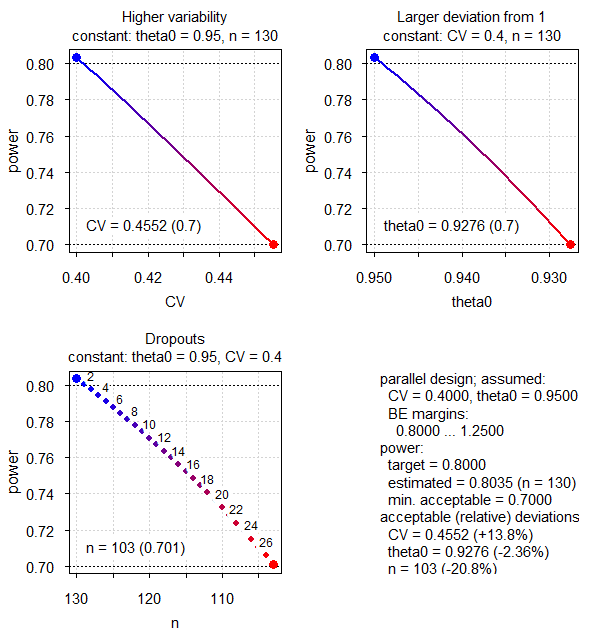

Fig. 1 Power analysis (CV 0.40, all defaults).

Since the sample size algorithm (modified Zhang’s method³) is quite efficient, in sampleN.TOST() we see just two rows in the sample size search. From the third panel in Fig. 1 we see that with 27 dropouts (103 eligible subjects, power 0.701) we will still maintain our minimum acceptable power. However, power for other sample sizes is difficult to judge.

If we want to get results also for unequal group sizes, we have to specify bal = FALSE in the script; otherwise, we would get only even sample sizes like in sampleN.TOST(). We have to specify also the design because the script’s default is a 2×2×2 crossover.
We use most of the script’s defaults applicable for this design: The nominal level of the test (alpha = 0.05), the assumed T/R-ratio (theta0 = 0.95), the BE margins (theta1 = 0.80, theta2 = 1.25), average BE (ABE = TRUE), exact power by Owen’s Q function⁴ (method = "exact"), target power (target = 0.8), minimum acceptable power (minpower = 0.7), no adjustment for dropouts (do.rate = 0), printing to the console (print = TRUE) and hence, we don’t have to specify these values. Although not necessary, I recommend to assign the result to a variable (here x). Then you can print the data frame, explore values, etc.

x <- power.table(CV = 0.4, design = "parallel", bal = FALSE)

# design        : parallel (two parallel groups) 
# alpha         : 0.0500 
# method        : Average Bioequivalence (ABE) 
# regulator     : all jurisdictions 
# power method  : exact 
# CVtotal       : 0.4000 
# theta0        : 0.9500 
# theta1        : 0.8000 
# theta2        : 1.2500 
# targetpower   : 0.8000 
# estimated n   : 130   (achieved power 0.80351) 
# minpower      : 0.7000 
# minimum n     : 103   (achieved power 0.70102) 
# 
#    n dropouts dropouts   power
#  130     none     none 0.80351
#  129        1   0.769% 0.80046
#  128        2   1.538% 0.79740
#  127        3   2.308% 0.79424
#  126        4   3.077% 0.79108
#  125        5   3.846% 0.78782
#  124        6   4.615% 0.78456
#  123        7   5.385% 0.78119
#  122        8   6.154% 0.77781
#  121        9   6.923% 0.77433
#  120       10   7.692% 0.77085
#  119       11   8.462% 0.76725
#  118       12   9.231% 0.76365
#  117       13  10.000% 0.75992
#  116       14  10.769% 0.75620
#  115       15  11.538% 0.75235
#  114       16  12.308% 0.74850
#  113       17  13.077% 0.74451
#  112       18  13.846% 0.74053
#  111       19  14.615% 0.73641
#  110       20  15.385% 0.73229
#  109       21  16.154% 0.72802
#  108       22  16.923% 0.72375
#  107       23  17.692% 0.71933
#  106       24  18.462% 0.71491
#  105       25  19.231% 0.71033
#  104       26  20.000% 0.70576
#  103       27  20.769% 0.70102

With the script’s default bal = TRUE we would get in the first two rows of the data frame the results of the sample search of sampleN.TOST(..., details = TRUE). All other results agree with pa.ABE() as well.
Since the script gives sample sizes and power (>= minpower and <= target), we see that with e.g., 16 dropouts or more (114 eligible subjects or less) power falls below 75%.

top of section ↩︎ previous section ↩︎

Crossover design

For background about sample size estimation see this article and for prospective power that one.

We assume a within-subject CV of 0.25 and apply all defaults.

x <- power.table(CV = 0.25)

# design        : 2x2x2 (conventional crossover) 
# alpha         : 0.0500 
# method        : Average Bioequivalence (ABE) 
# regulator     : all jurisdictions 
# power method  : exact 
# CVw           : 0.2500 
# theta0        : 0.9500 
# theta1        : 0.8000 
# theta2        : 1.2500 
# targetpower   : 0.8000 
# estimated n   : 28    (achieved power 0.80744) 
# minpower      : 0.7000 
# minimum n     : 24    (achieved power 0.73912) 
# 
#   n dropouts dropouts   power
#  28     none     none 0.80744
#  26        2   7.143% 0.77606
#  24        4  14.286% 0.73912

Agrees with what we would obtain in sampleN.TOST(..., details = TRUE).

If the variability is small, we may end up with a sample size which is below the regulatory minimum. The script notifies us about that.

x <- power.table(CV = 0.15, bal = FALSE)

# Note: If there will be at least one dropout, less than 
#       12 eligible subjects; consider to increase the 
#       sample size in a pivotal study.

# design        : 2x2x2 (conventional crossover) 
# alpha         : 0.0500 
# method        : Average Bioequivalence (ABE) 
# regulator     : all jurisdictions 
# power method  : exact 
# CVw           : 0.1500 
# theta0        : 0.9500 
# theta1        : 0.8000 
# theta2        : 1.2500 
# targetpower   : 0.8000 
# estimated n   : 12    (achieved power 0.83052) 
# minpower      : 0.7000 
# minimum n     : 10    (achieved power 0.74151) 
# 
#   n dropouts dropouts   power
#  12     none     none 0.83052
#  11        1   8.333% 0.78774
#  10        2  16.667% 0.74151

It is common to adjust the sample size for the anticipated dropout-rate. When using sampleN.TOST() you would have to do the calculation manually or use the functions given in another article.
Let’s assume 5% of dropouts.

x <- power.table(CV = 0.15, do.rate = 0.05, bal = FALSE)

# Note: If there will be more than 2 dropouts, less than 
#       12 eligible subjects; consider to increase the 
#       sample size in a pivotal study.

# design        : 2x2x2 (conventional crossover) 
# alpha         : 0.0500 
# method        : Average Bioequivalence (ABE) 
# regulator     : all jurisdictions 
# power method  : exact 
# CVw           : 0.1500 
# theta0        : 0.9500 
# theta1        : 0.8000 
# theta2        : 1.2500 
# targetpower   : 0.8000 
# estimated n   : 12    (achieved power 0.83052) 
# dropout-rate  :  5.0% (anticipated) 
# adjusted n    : 14    (achieved power 0.88798) 
# minpower      : 0.7000 
# minimum n     : 12    (achieved power 0.83052) 
# 
#   n dropouts dropouts   power
#  14     none     none 0.88798
#  13        1   7.143% 0.86037
#  12        2  14.286% 0.83052

If you want to be on the safe side, opt for an even larger sample size. We don’t want to end up with less eligible subjects than the regulatory minimum.

For highly variable C_max a fixed BE-range of 75.00 – 133.33% is acceptable.⁵ ⁶ Contrary to SABE in other jurisdictions, a replicate design is not required. Let’s assume CV 0.45 and a – for HVD(P)s realistic⁷ – T/R-ratio 0.9. By specifiying theta1 = 0.75 the upper limit theta2 is automatically calculated.

x <- power.table(CV = 0.45, theta0 = 0.9, theta1 = 0.75)

# design        : 2x2x2 (conventional crossover) 
# alpha         : 0.0500 
# method        : Average Bioequivalence (ABE) 
# regulator     : all jurisdictions 
# power method  : exact 
# CVw           : 0.4500 
# theta0        : 0.9000 
# theta1        : 0.7500 
# theta2        : 1.3333 
# targetpower   : 0.8000 
# estimated n   : 72    (achieved power 0.80991) 
# minpower      : 0.7000 
# minimum n     : 54    (achieved power 0.70164) 
# 
#   n dropouts dropouts   power
#  72     none     none 0.80991
#  70        2   2.778% 0.79996
#  68        4   5.556% 0.78954
#  66        6   8.333% 0.77864
#  64        8  11.111% 0.76722
#  62       10  13.889% 0.75528
#  60       12  16.667% 0.74277
#  58       14  19.444% 0.72969
#  56       16  22.222% 0.71599
#  54       18  25.000% 0.70164

In a 2-sequence 4-period full replicate design we would require 36 subjects as for the GCC’s approach. Compare that to the 28 subjects for ABEL and the 24 for RSABE. More about that below.

top of section ↩︎ previous section ↩︎

Replicate designs

For background about sample size estimation see this article.

If we want to design a study intended for reference-scaling by ABEL (see below), in most jurisdictions⁸ we have to assess AUC still for ABE because expanding the limits is acceptable only for C_max. If AUC is highly variable as well, commonly it drives the sample size.

Let’s assume CV 0.45 and a T/R-ratio of 0.9 in a 2-sequence 4-period full replicate design. Due to more periods, the chance of dropouts is higher than in a conventional 2×2×2 crossover and hence, we anticipate a dropout-rate of 10%.

x <- power.table(CV = 0.45, theta0 = 0.9, design = "2x2x4", do.rate = 0.1, bal = FALSE)

# design        : 2x2x4 (2-sequence 4-period full replicate) 
# alpha         : 0.0500 
# method        : Average Bioequivalence (ABE) 
# regulator     : all jurisdictions 
# power method  : exact 
# CVw           : 0.4500 
# theta0        : 0.9000 
# theta1        : 0.8000 
# theta2        : 1.2500 
# targetpower   : 0.8000 
# estimated n   : 84    (achieved power 0.80569) 
# dropout-rate  : 10.0% (anticipated) 
# adjusted n    : 94    (achieved power 0.84326) 
# minpower      : 0.7000 
# minimum n     : 64    (achieved power 0.70592) 
# 
#   n dropouts dropouts   power
#  94     none     none 0.84326
#  93        1   1.064% 0.83978
#  92        2   2.128% 0.83632
#  91        3   3.191% 0.83270
#  90        4   4.255% 0.82910
#  89        5   5.319% 0.82534
#  88        6   6.383% 0.82159
#  87        7   7.447% 0.81768
#  86        8   8.511% 0.81379
#  85        9   9.574% 0.80973
#  84       10  10.638% 0.80569
#  83       11  11.702% 0.80147
#  82       12  12.766% 0.79728
#  81       13  13.830% 0.79290
#  80       14  14.894% 0.78854
#  79       15  15.957% 0.78399
#  78       16  17.021% 0.77947
#  77       17  18.085% 0.77475
#  76       18  19.149% 0.77006
#  75       19  20.213% 0.76516
#  74       20  21.277% 0.76031
#  73       21  22.340% 0.75522
#  72       22  23.404% 0.75019
#  71       23  24.468% 0.74492
#  70       24  25.532% 0.73970
#  69       25  26.596% 0.73423
#  68       26  27.660% 0.72883
#  67       27  28.723% 0.72317
#  66       28  29.787% 0.71757
#  65       29  30.851% 0.71171
#  64       30  31.915% 0.70592

Such an extreme sample size is a nasty side effect of not being allowed to apply reference-scaling. For ABEL we would require only 28 subjects and for RSABE just 24…
If we are lucky and have eleven dropouts or less (83 eligible subjects or more), power will be at least our target of 80%.

top of section ↩︎ previous section ↩︎

Reference-scaling

ABEL

Applicable for the EMA and others. For background about sample size estimation see this article and for prospective power that one.

We assume homoscedasticity (CV_wT = CV_wR = 0.3) and apply the defaults of the script. In order to employ SABE, we specify ABE = FALSE.

x <- power.table(CV = 0.3, ABE = FALSE)

# design        : 2x3x3 (3-sequence 3-period ‘partial’ replicate) 
# alpha         : 0.0500 
# regulator     : EMA and others 
# method        : Average Bioequivalence with Expanding Limits (ABEL) 
# simulations   : ANOVA 
#   number      : 100,000 
# CVswitch      : 0.3000 
# Reg. constant : 0.76 
# PE constraints: 0.8000, 1.2500 
# Cap           : 0.5000 
# CVwT = CVwR   : 0.3000 
# theta0        : 0.9000 
# theta1        : 0.8000 
# theta2        : 1.2500 
# targetpower   : 0.8000 
# estimated n   : 54    (achieved power 0.81593) 
# minpower      : 0.7000 
# minimum n     : 39    (achieved power 0.70777) 
# 
#   n dropouts dropouts   power
#  54     none     none 0.81593
#  51        3   5.556% 0.79859
#  48        6  11.111% 0.77839
#  45        9  16.667% 0.75710
#  42       12  22.222% 0.73305
#  39       15  27.778% 0.70777

As an aside, at CV_wR = 0.3 we may not expand the limits⁹ and hence, the conventional BE margins have to be used.

Whilst sampleN.scABEL() supports heteroscedasticity (CV_wT ≠ CV_wR), pa.scABE() does not.
Let’s keep (the pooled) CV_w at 0.3 but assume that the test product is less variable (CV_wT 0.2822) than the reference (CV_wR 0.3170), i.e., the ratio of variances is 0.8.

CV <- signif(CVp2CV(0.3, ratio = 0.8), 4)
x  <- power.table(CV = CV, ABE = FALSE)

# design        : 2x3x3 (3-sequence 3-period ‘partial’ replicate) 
# alpha         : 0.0500 
# regulator     : EMA and others 
# method        : Average Bioequivalence with Expanding Limits (ABEL) 
# simulations   : ANOVA 
#   number      : 100,000 
# CVswitch      : 0.3000 
# Reg. constant : 0.76 
# PE constraints: 0.8000, 1.2500 
# Cap           : 0.5000 
# CVwT          : 0.2822 
# CVwR          : 0.3170 
# theta0        : 0.9000 
# L, U          : 0.7904, 1.2651 
# targetpower   : 0.8000 
# estimated n   : 48    (achieved power 0.80164) 
# minpower      : 0.7000 
# minimum n     : 36    (achieved power 0.70471) 
# 
#   n dropouts dropouts   power
#  48     none     none 0.80164
#  45        3   6.250% 0.78101
#  42        6  12.500% 0.75832
#  39        9  18.750% 0.73240
#  36       12  25.000% 0.70471

Since CV_wR 31.70% > 30%, we may expand the limits slighly to 0.7904 – 1.2651. Hence, we require a lower sample size than in the previous example.

Health Canada¹⁰ accepts ABEL only for AUC (the point estimate of C_max has to lie within 80.0 – 125.0%). Similar than above for simplicity. We have to use the argument regulator.

CV <- signif(CVp2CV(0.3, ratio = 0.8), 4)
x  <- power.table(CV = CV, ABE = FALSE, regulator = "HC")

# design        : 2x3x3 (3-sequence 3-period ‘partial’ replicate) 
# alpha         : 0.0500 
# regulator     : Health Canada 
# method        : Average Bioequivalence with Expanding Limits (ABEL) 
# simulations   : intra-subject contrasts 
#   number      : 100,000 
# CVswitch      : 0.3000 
# Reg. constant : 0.76 
# PE constraints: 0.8000, 1.2500 
# Cap           : 0.5738 
# CVwT          : 0.2822 
# CVwR          : 0.3170 
# theta0        : 0.9000 
# L, U          : 0.7904, 1.2651 
# targetpower   : 0.8000 
# estimated n   : 48    (achieved power 0.81432) 
# minpower      : 0.7000 
# minimum n     : 36    (achieved power 0.71621) 
# 
#   n dropouts dropouts   power
#  48     none     none 0.81432
#  45        3   6.250% 0.79188
#  42        6  12.500% 0.76889
#  39        9  18.750% 0.74356
#  36       12  25.000% 0.71621

Pretty similar to the previous example (48 subjects, power 0.81432 > 0.80164 for the EMA). Larger differences would be observed for higher variabilities, mainly due to the different cap of scaling (~57.4% for Health Canada and 50% for the other jurisdictions).

We know that in SABE the Type I Error (TIE) can be inflated¹¹ (for details see another article). The script supports such an assessment as well. Assessing the first example by using the argument TIE. This time we suppress the details and print only the data frame.

x <- power.table(CV = 0.3, ABE = FALSE, TIE = TRUE, details = FALSE)
print(x, row.names = FALSE)

# Patience please. Simulating empiric Type I Error is time consuming.
#   n dropouts dropouts   power      TIE infl
#  54     none     none 0.81593 0.071891  yes
#  51        3   5.556% 0.79859 0.071573  yes
#  48        6  11.111% 0.77839 0.071592  yes
#  45        9  16.667% 0.75710 0.071179  yes
#  42       12  22.222% 0.73305 0.071121  yes
#  39       15  27.778% 0.70777 0.070930  yes

We get two additional columns. The first gives the empiric Type I Error obtained by one million simulations under the Null and the second one shows whether the TIE is significantly inflated (i.e., above the limit of the binomial test of 0.05036). Such a result is not surprising, since the maximum inflation is always observed at the switching CV_wR of 30%.

Depending on the design and approach, the area of inflated Type I Errors is limited at a certain CV_wR (generally < 45%) and depends on the sample size as well…

x <- power.table(CV = 0.44, ABE = FALSE, design = "2x2x4", bal = FALSE,
                 TIE = TRUE, details = FALSE)
print(x, row.names = FALSE)

# Patience please. Simulating empiric Type I Error is time consuming.
#   n dropouts dropouts   power      TIE infl
#  28     none     none 0.80735 0.051681  yes
#  27        1   3.571% 0.79520 0.051431  yes
#  26        2   7.143% 0.78167 0.051330  yes
#  25        3  10.714% 0.76606 0.051062  yes
#  24        4  14.286% 0.75059 0.050670  yes
#  23        5  17.857% 0.73271 0.050003  no 
#  22        6  21.429% 0.71591 0.049486  no

A special case is the approach of the Gulf Cooperation Council (GCC), where the limits are not scaled but directly widened to 75.00 – 133.33% for any CV_wR > 30%.¹²

CV <- signif(CVp2CV(0.3, ratio = 0.8), 4)
x  <- power.table(CV = CV, ABE = FALSE, regulator = "GCC")

# design        : 2x3x3 (3-sequence 3-period ‘partial’ replicate) 
# alpha         : 0.0500 
# regulator     : Gulf Cooperation Council 
# method        : Average Bioequivalence with widened limits 
# simulations   : ANOVA 
#   number      : 100,000 
# CVswitch      : 0.3000 
# Reg. constant : 0.9799758 
# PE constraints: 0.8000, 1.2500 
# CVwT          : 0.2822 
# CVwR          : 0.3170 
# theta0        : 0.9000 
# L, U          : 0.7500, 1.3333 
# targetpower   : 0.8000 
# estimated n   : 36    (achieved power 0.80613) 
# minpower      : 0.7000 
# minimum n     : 27    (achieved power 0.70272) 
# 
#   n dropouts dropouts   power
#  36     none     none 0.80613
#  33        3   8.333% 0.77693
#  30        6  16.667% 0.74156
#  27        9  25.000% 0.70272

We need a substantially lower sample size than in ABEL (48 subjects), where the expanded limits would be narrower (0.7904 – 1.2651).

top of section ↩︎ previous section ↩︎

RSABE

Applicable for the FDA¹³ and China’s CDE.¹⁴

HVD(P)s

For background about sample size estimation see this article and for prospective power that one.

CV <- signif(CVp2CV(0.6, ratio = 0.8), 4)
x  <- power.table(CV = CV, design = "2x2x4", ABE = FALSE,
                  regulator = "FDA", bal = FALSE)

# design        : 2x2x4 (2-sequence 4-period full replicate) 
# alpha         : 0.0500 
# regulator     : FDA or CDE 
# method        : Reference-scaled Average Bioequivalence (RSABE) 
# simulations   : intra-subject contrasts 
#   number      : 100,000 
# CVswitch      : 0.3000 
# Reg. constant : 0.8925742 
# PE constraints: 0.8000, 1.2500 
# CVwT          : 0.5606 
# CVwR          : 0.6382 
# theta0        : 0.9000 
# Implied limits: 0.5935, 1.6849 
# targetpower   : 0.8000 
# estimated n   : 22    (achieved power 0.81038) 
# adjusted n    : 24    (achieved power 0.83100) 
#                 increased to comply with regulatory minimum 
# minpower      : 0.7000 
# minimum n     : 16    (achieved power 0.70537) 
# 
#   n dropouts dropouts   power
#  24     none     none 0.83100
#  23        1   4.167% 0.82127
#  22        2   8.333% 0.81038
#  21        3  12.500% 0.79855
#  20        4  16.667% 0.78519
#  19        5  20.833% 0.76817
#  18        6  25.000% 0.75153
#  17        7  29.167% 0.72886
#  16        8  33.333% 0.70537

Contrary to other jurisdictions, where guidelines specify a minimum number of eligible subjects, the FDA requires 24 dosed subjects if the study is designed for RSABE. Though it is overly optimistic to assume no dropouts in a design with four periods, the script increases the sample size if the estimated one is too low.

top of section ↩︎ previous section ↩︎

NTIDs

Applicable for the FDA¹³ ¹⁵ ¹⁶ ¹⁷ and China’s CDE.¹⁴

For background about sample size estimation see this article and for prospective power that one.

The approach consists of assessing three components: RSABE (95% CI of the scaled criterion ≤ 0), conventional ABE (90% CI within 80.00 – 125.00%), and the upper CL of \(\small{\sigma_\text{wT}/\sigma_\text{wR}}\) ≤ 2.5. If \(\small{s_\text{wT}>s_\text{wR}}\) the impact on power and hence, the sample size can be substantial. The script gives three additional columns showing the power of the components.

Here an example where the test product is more variable (CV_wT 0.1181) than the reference (CV_wR 0.0786), i.e., the ratio of variances is 2.25 (\(\small{s_\text{wT}/s_\text{wT}=1.5}\)).

CV <- se2CV(0.1) # at the switching standard deviation 0.1
CV <- signif(CVp2CV(CV, ratio = 2.25), 4)
x  <- power.table(CV = CV, NTID = TRUE, do.rate = 0.1, bal = FALSE)

# design        : 2x2x4 (2-sequence 4-period full replicate) 
# alpha         : 0.0500 
# regulator     : FDA or CDE 
# method        : RSABE (NTID) 
# simulations   : intra-subject contrasts 
#   number      : 100,000 
# Reg. constant : 1.053605 
# ‘Cap’         : 0.2142 
# Implied limits: 0.9207, 1.0862 
# ABE limits    : 0.8000, 1.2500 
# CVwT          : 0.1181 
# CVwR          : 0.0786 
# theta0        : 0.9750 
# targetpower   : 0.8000 
# estimated n   : 34    (achieved power 0.80635) 
# dropout-rate  : 10.0% (anticipated) 
# adjusted n    : 38    (achieved power 0.85482) 
# minpower      : 0.7000 
# minimum n     : 28    (achieved power 0.71021) 
# 
#   n dropouts dropouts   power   RSABE ABE s-ratio
#  38     none     none 0.85482 0.92086   1 0.91709
#  37        1   2.632% 0.84381 0.91306   1 0.91050
#  36        2   5.263% 0.83260 0.90749   1 0.90206
#  35        3   7.895% 0.82023 0.90016   1 0.89451
#  34        4  10.526% 0.80635 0.89210   1 0.88592
#  33        5  13.158% 0.79408 0.88392   1 0.87832
#  32        6  15.789% 0.77761 0.87515   1 0.86744
#  31        7  18.421% 0.76204 0.86324   1 0.85747
#  30        8  21.053% 0.74602 0.85412   1 0.84631
#  29        9  23.684% 0.72733 0.84341   1 0.83235
#  28       10  26.316% 0.71021 0.83185   1 0.81988

We see that the \(\small{\sigma_\text{wT}/\sigma_\text{wR}}\)-test has the lowest power and therefore, drives the sample size.

Let’s compare that to fixed narrower limits of 90.00 – 111.11% for NTIDs recommended in all other jurisdictions.¹⁸ It must be mentioned that the conventional model of ABE assumes homoscedasticity \(\small{(s_\text{wT}^2=s_\text{wR}^2)}\).

CV <- se2CV(0.1) # ≈10.02505%
x  <- power.table(CV = CV, theta1 = 0.9, design = "2x2x4",
                  do.rate = 0.1, bal = FALSE)

# Note: If there will be more than 2 dropouts, less than 
#       12 eligible subjects; consider to increase the 
#       sample size in a pivotal study.

# design        : 2x2x4 (2-sequence 4-period full replicate) 
# alpha         : 0.0500 
# method        : Average Bioequivalence (ABE); NTID 
# regulator     : EMA and others 
# power method  : exact 
# CVw           : 0.1003 
# theta0        : 0.9750 
# theta1        : 0.9000 
# theta2        : 1.1111 
# targetpower   : 0.8000 
# estimated n   : 12    (achieved power 0.85467) 
# dropout-rate  : 10.0% (anticipated) 
# adjusted n    : 14    (achieved power 0.90172) 
# minpower      : 0.7000 
# minimum n     : 12    (achieved power 0.85467) 
# 
#   n dropouts dropouts   power
#  14     none     none 0.90172
#  13        1   7.143% 0.87871
#  12        2  14.286% 0.85467

To achieve our target power we require substantially less subjects than with RSABE (12 instead of 34). Let’s assume homoscedasticity.

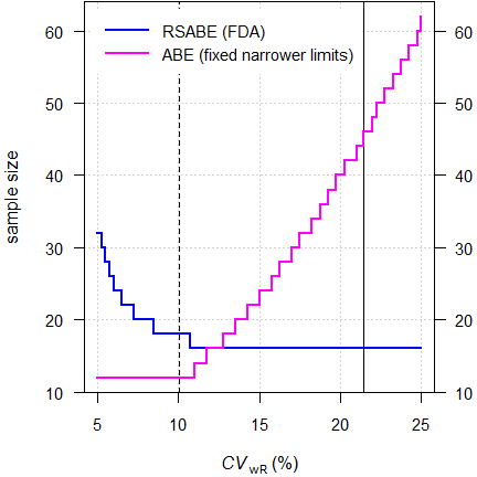
Fig. 2 Sample sizes for RSABE vs. ABE with fixed narrower limits.
2-sequence 4-period full replicate design, assumed T/R-ratio 0.975
targeted at ≥ 80% power, homoscedasticity (\(\small{s_\text{wT}^2=s_\text{wR}^2}\)).

Smaller sample sizes for ABE with fixed narrower limits are obtained for relatively small variabilities. With larger variabilities, sample sizes increase quickly.

In RSABE heteroscedasticity can be challenging if \(\small{s_\text{wT}^2 > s_\text{wR}^2}\).

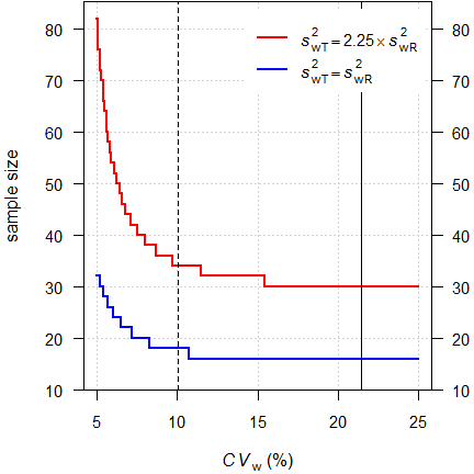
Fig. 3 Sample sizes for RSABE.
2-sequence 4-period full replicate design, assumed T/R-ratio 0.975
targeted at ≥ 80% power, homo- and heteroscedasticity.

With homoscedasticity we would need only 18 subjecs instead of 34 to achieve our target power.

top of section ↩︎ previous section ↩︎

Licenses

Helmut Schütz 2022
R and PowerTOST GPL 3.0, klippy MIT, pandoc GPL 2.0.
1^st version October 24, 2022. Rendered October 28, 2022 14:12 CEST by rmarkdown via pandoc in 2.34 seconds.

Footnotes and References

Labes D, Schütz H, Lang B. PowerTOST: Power and Sample Size for (Bio)Equivalence Studies. Package version 1.5.4.9000. 2022-04-25. CRAN.↩︎
Achievwin. R code for Average BE or parallel design N computations. BEBA-Forum. Vienna. 2022-09-16. Online.↩︎
Zhang P. A Simple Formula for Sample Size Calculation in Equivalence Studies. J Biopharm Stat. 2003; 13(3): 529–38. doi:10.1081/BIP-120022772.↩︎
Owen DB. A special case of a bivariate non-central t-distribution. Biometrika. 1965; 52(3/4): 437–46. doi:10.2307/2333696.↩︎
League of Arab States, Higher Technical Committee for Arab Pharmaceutical Industry. Harmonised Arab Guideline on Bioequivalence of Generic Pharmaceutical Products. Cairo. March 2014. Online.↩︎
Medicines Control Council. Registration of Medicines: Biostudies. Pretoria. June 2015. Online.↩︎
Tóthfalusi L, Endrényi L. Sample Sizes for Designing Bioequivalence Studies for Highly Variable Drugs. J Pharm Pharmacol Sci. 2012; 15(1): 73–84. doi:10.18433/j3z88f. Open Access.↩︎
Except for the WHO, where ABEL is acceptable for both C_max and AUC and modified release products for the EMA, where ABEL is acceptable for partial AUCs.↩︎
The probability that we may expand the limits is approximately 50%. Therefore, in ABEL the sample size is smaller than in ABE. Try fixed limits:
sampleN.TOST(CV = 0.3, theta0 = 0.9, design = "2x3x3")↩︎
Health Canada. Guidance Document. Comparative Bioavailability Standards: Formulations Used for Systemic Effects. Ottawa. 08 June 2018. Online.↩︎
Schütz H, Labes D, Wolfsegger MJ. Critical Remarks on Reference-Scaled Average Bioequivalence. J Pharm Pharmaceut Sci. 25: 285–96. doi:10.18433/jpps32892.↩︎
Executive Board of the Health Ministers’ Council for GCC States. The GCC Guidelines for Bioequivalence. May 2021. Online.↩︎
FDA, CDER. Draft Guidance for Industry. Bioequivalence Studies with Pharmacokinetic Endpoints for Drugs Submitted Under an ANDA. Silver Spring. August 2021. Download.↩︎
CDE. Annex 2. Technical guidelines for research on bioequivalence of highly variable drugs. Download. [Chinese].↩︎
FDA, OGD. Guidance on Warfarin Sodium. Rockville. Recommended Dec 2012. Download.↩︎
Endrényi L, Tóthfalusi L. Determination of Bioequivalence for Drugs with Narrow Therapeutic Index: Reduction of the Regulatory Burden. J Pharm Pharm Sci. 2013; 16(5): 676–82. Open Access.↩︎
Yu LX, Jiang W, Zhang X, Lionberger R, Makhlouf F, Schuirmann DJ, Muldowney L, Chen ML, Davit B, Conner D, Woodcock J. Novel bioequivalence approach for narrow therapeutic index drugs. Clin Pharmacol Ther. 2015; 97(3): 286–91. doi:10.1002/cpt.28.↩︎
Depending on the drug only AUC or C_max or both. See the respective product-specific guidance.↩︎