
Sample Size Estimation for Equivalence Studies Intended for RSABE
Helmut Schütz
June 21, 2023
Consider allowing JavaScript. Otherwise, you have to be proficient in
reading  since formulas
will not be rendered. Furthermore, the table of contents in the left
column for navigation will not be available and code-folding not
supported. Sorry for the inconvenience.
since formulas
will not be rendered. Furthermore, the table of contents in the left
column for navigation will not be available and code-folding not
supported. Sorry for the inconvenience.
Examples in this article were generated with
 4.3.1
by the package
4.3.1
by the package PowerTOST.1
More examples are given in the respective vignette.2 See also the README on GitHub for an overview and the online manual3 for details.
- The right-hand badges give the respective section’s ‘level’.
- Basics about sample size methodology – requiring no or only limited statistical expertise.
- These sections are the most important ones. They are – hopefully – easily comprehensible even for novices.
- A somewhat higher knowledge of statistics and/or R is required. May be skipped or reserved for a later reading.
- An advanced knowledge of statistics and/or R is required. Not recommended for beginners in particular.
- If you are not a neRd or statistics afficionado, skipping is recommended. Suggested for experts but might be confusing for others.
- Click to show / hide R code. float-right”>Code
- Click on the icon
 in the top left corner to copy R code to the
clipboard.
in the top left corner to copy R code to the
clipboard.
| Abbreviation | Meaning |
|---|---|
| \(\small{\alpha}\) | Nominal level of the test, probability of Type I Error (patient’s risk) |
| (A)BE | (Average) Bioequivalence |
| ABEL | Average Bioequivalence with Expanding Limits |
| \(\small{\beta}\) | Probability of Type II Error (producer’s risk), where \(\small{\beta=1-\pi}\) |
| \(\small{CV_\text{b}}\) | Between-subject Coefficient of Variation |
| \(\small{CV_\text{w}}\) | (Pooled) within-subject Coefficient of Variation |
| \(\small{CV_\text{wR},\;CV_\text{wT}}\) | Observed within-subject Coefficient of Variation of the Reference and Test product |
| \(\small{H_0}\) | Null hypothesis (inequivalence) |
| \(\small{H_1}\) | Alternative hypothesis (equivalence) |
| \(\small{\mu_\text{T}/\mu_\text{R}}\) | True T/R-ratio |
| HVD(P) | Highly Variable Drug (Product) |
| \(\small{\pi}\) | (Prospective) power, where \(\small{\pi=1-\beta}\) |
| PE | Point Estimate |
| R | Reference product |
| RSABE | Reference-scaled Average Bioequivalence |
| SABE | Scaled Average Bioequivalence |
| \(\small{s_\text{bR}^2,\;s_\text{bT}^2}\) | Observed between-subject variance of the Reference and Test product |
| \(\small{s_\text{wR},\;s_\text{wT}}\) | Observed within-subject standard deviation of the Reference and Test product |
| \(\small{s_\text{wR}^2,\;s_\text{wT}^2}\) | Observed within-subject variance of the Reference and Test product |
| \(\small{\sigma_\text{wR}}\) | True within-subject standard deviation of the Reference product |
| T | Test product |
| \(\small{\theta_0}\) | True T/R-ratio |
| \(\small{\theta_1,\;\theta_2}\) | Fixed lower and upper limits of the acceptance range (generally 80.00 – 125.00%) |
| \(\theta_\text{s}\) | Regulatory constant (≈0.8925742…) |
| \(\small{\theta_{\text{s}_1},\;\theta_{\text{s}_2}}\) | Scaled lower and upper limits of the acceptance range |
| TIE | Type I Error (patient’s risk) |
| TIIE | Type II Error (producer’s risk: 1 – power) |
Introduction
What is Reference-scaled Average Bioequivalence?
For details about inferential statistics and hypotheses in equivalence see another article.
Definitions:
- A Highy Variable Drug (HVD) shows a within-subject Coefficient of Variation (CVwR) > 30% if administered as a solution in a replicate design. The high variability is an intrinsic property of the drug (absorption/permeation, clearance).
- A Highy Variable Drug Product (HVDP) shows a CVwR > 30% in a replicate design.4
The concept of Scaled Average Bioequivalence (SABE) for HVD(P)s is based on the following considerations:
- HVD(P)s are safe and efficacious despite their high variability
because:
- They have a wide therapeutic index (i.e., a flat
dose-response curve). Consequently, even substantial changes in
concentrations have only a limited impact on the effect.
If they would have a narrow therapeutic index, adverse effects (due to high concentrations) and lacking effects (due to low concentrations) would have been observed in Phase III and consequently, the originator’s product not be approved in the first place. - Once approved, the product has a documented safety / efficacy record
in phase IV and in clinical practice – despite its high
variability.
If problems were evident, the product would have been taken off the market.
- They have a wide therapeutic index (i.e., a flat
dose-response curve). Consequently, even substantial changes in
concentrations have only a limited impact on the effect.
- Given that, the conventional ‘clinically relevant difference’ Δ of 20% (leading to the limits of 80.00 – 125.00% in Average Bioequivalence) is overly conservative and thus, leading to large sample sizes.
- Hence, a more relaxed Δ of > 20% was proposed. A natural approach is to scale the limits based on the within-subject variability of the reference product σwR. In this approach, power for a given sample size is essentially independent from the variability (see Fig. 4).
The conventional confidence interval inclusion approach in ABE \[\begin{matrix}\tag{1} \theta_1=1-\Delta,\theta_2=\left(1-\Delta\right)^{-1}\\ H_0:\;\frac{\mu_\text{T}}{\mu_\text{R}}\ni\left\{\theta_1,\,\theta_2\right\}\;vs\;H_1:\;\theta_1<\frac{\mu_\text{T}}{\mu_\text{R}}<\theta_2, \end{matrix}\] where \(\small{H_0}\) is the null hypothesis of inequivalence and \(\small{H_1}\) the alternative hypothesis, \(\small{\theta_1}\) and \(\small{\theta_2}\) are the fixed lower and upper limits of the acceptance range, and \(\small{\mu_\text{T}}\) are the geometric least squares means of \(\small{\text{T}}\) and \(\small{\text{R}}\), respectively, is in Scaled Average Bioequivalence (SABE)5 6 modified to \[H_0:\;\frac{\mu_\text{T}}{\mu_\text{R}}\Big{/}\sigma_\text{wR}\ni\left\{\theta_{\text{s}_1},\,\theta_{\text{s}_2}\right\}\;vs\;H_1:\;\theta_{\text{s}_1}<\frac{\mu_\text{T}}{\mu_\text{R}}\Big{/}\sigma_\text{wR}<\theta_{\text{s}_2},\tag{2}\] where \(\small{\sigma_\text{wR}}\) is the standard deviation of the reference and the scaled limits \(\small{\left\{\theta_{\text{s}_1},\,\theta_{\text{s}_2}\right\}}\) of the acceptance range depend on conditions given by the agency.
Reference-Scaled Average Bioequivalence (RSABE) for HVD(P)s is recommended by the FDA7 8 and China’s CDE.9
Alas, we are far away from global harmonization. Average Bioequivalence with Expanding Limits (ABEL) is another variant of SABE and recommended in all other jurisdictions accepting SABE. See another article for details.
In order to apply RSABE following conditions have to be fulfilled:
- The study has to be performed in a replicate design (i.e., at least the reference product has to be administered twice).
- The observed within-subject standard deviation of the reference swR has to be ≥ 0.294 (CVwR ≥ ≈0.30047).
The approach given in the guidances7 8 9 is a decision scheme which hinges on the estimated standard deviation of the reference treatment \(\small{s_{\text{wR}}}\). If \(\small{s_\text{wR}<0.294}\) the study has to be assessed for ABE (left branch) and for RSABE (right branch) otherwise. In the RSABE-branch the point estimate (\(\small{PE}\)) has to lie within 80.00 – 125.00%.
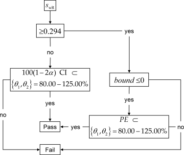
Fig. 1 Decision scheme.
Based on the switching standard deviation \(\small{s_0=0.25}\) we get the regulatory constant \(\small{\theta_\text{s}=\frac{\log_{e}1.25}{s_0}=0.8925742\ldots}\) and finally the ‘implied limits’ \(\small{\left\{\theta_{\text{s}_1},\theta_{\text{s}_2}\right\}=100\left(\exp(\mp0.8925742\cdot s_{\text{wR}})\right)}\).13
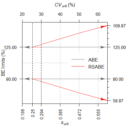
Fig. 2 ‘Implied limits’
depending on the observed \(\small{s_{\text{wR}}}\).
Dashed
vertical lines at the switching condition and the applicable lower cap
of scaling.
Note that scaling starts at the switching standard deviation \(\small{s_0=0.25}\) (\(\small{CV_0\approx25.396\%}\)) but according to the guidances7 8 9 must be only applied if \(\small{s_{\text{wR}}\geq0.294}\) (\(\small{CV_{\text{wR}}\geq\approx0.30047}\)), thus explaining the dichotomy14 at this value.
Note also that – contrary to ABEL – there is no upper cap of scaling. However, for very large variability the decision is mainly lead by the \(\small{PE}\)-constraint.
Since the applicability of this approach depends on the realized values (\(\small{s_\text{wR}}\), \(\small{PE}\)) in the particular study – which are naturally unknown beforehand – analytical solutions for power (and hence, the sample size) do not exist. Therefore, extensive simulations of potential combinations have to be employed.
Cave: If \(\small{s_{\text{wR}}<0.294}\) the method may lead to an inflated Type I Error (increased patient’s risk). It is elaborated in another article.
Preliminaries
A basic knowledge of R is
required. To run the scripts at least version 1.4.8 (2019-08-29) of
PowerTOST is required and at least version 1.5.3
(2021-01-18) suggested. Any version of R would
likely do, though the current release of PowerTOST was only
tested with version 4.1.3 (2022-03-10) and later. All scripts were run
on a Xeon E3-1245v3 @ 3.40GHz (1/4 cores) 16GB RAM with R 4.3.1 on Windows 7.
Note that in all functions of PowerTOST the arguments
(say, the assumed T/R-ratio theta0, the assumed coefficient
of variation CV, etc.) have to be given as ratios and not
in percent.
sampleN.RSABE() gives balanced sequences (i.e.,
an equal number of subjects is allocated to all sequences). Furthermore,
the estimated sample size is the total number of subjects.
All examples deal with studies where the response variables likely follow a log-normal distribution, i.e., we assume a multiplicative model (ratios instead of differences). We work with \(\small{\log_{e}}\)-transformed data in order to allow analysis by the t-test (requiring differences).
Terminology
It may sound picky but ‘sample size calculation’ (as used in most guidelines and alas, in some publications and textbooks) is sloppy terminology. In order to get prospective power (and hence, a sample size), we need five values:
- The level of the test \(\small{\alpha}\) (in BE commonly 0.05),
- the (potentially) expanded/widened BE-margin,
- the desired (or target) power \(\small{\pi}\),
- the variance (commonly expressed as a coefficient of variation), and
- the deviation of the test from the reference treatment,
where
- is fixed by the agency,
- depends on the observed15 \(\small{CV_\text{wR}}\) (which is unknown beforehand),
- is set by the sponsor (commonly to 0.80 – 0.90),
- is an uncertain assumption,
- is an uncertain assumption.
In other words, obtaining a sample size is not an exact calculation like \(\small{2\times2=4}\) but always just an estimation.
“Power Calculation – A guess masquerading as mathematics.
Of note, it is extremely unlikely that all assumptions will be exactly realized in a particular study. Hence, calculating retrospective (a.k.a. post hoc, a posteriori) power is not only futile but plain nonsense.17
Since generally the within-subject variability \(\small{CV_\text{w}}\) is smaller than the between-subject variability \(\small{CV_\text{b}}\), crossover studies are so popular. Of note, there is no relationship between \(\small{CV_\text{w}}\) and \(\small{CV_\text{b}}\). An example are drugs which are subjected to polymorphic metabolism. For these drugs \(\small{CV_\text{w}\ll CV_\text{b}}\).
Furthermore, the drugs’ within-subject variability may be unequal (i.e., \(\small{s_{\text{wT}}^{2}\neq s_{\text{wR}}^{2}}\)). For details see the section Heteroscedasticity.
It is a prerequisite that no carryover from one period to the next exists. Only then the comparison of treatments will be unbiased.18 Carryover is elaborated in another article.
For neRs only!
Power → Sample size
The sample size cannot be
directly estimated,
in SABE only power
simulated for an already given sample size.
“Power. That which statisticians are always calculating but never have.
Let’s start with PowerTOST.
library(PowerTOST) # attach it to run the examplesThe sample size functions’ defaults are:
| Argument | Default | Meaning |
|---|---|---|
alpha
|
0.05
|
Nominal level of the test. |
targetpower
|
0.80
|
Target (desired) power. |
theta0
|
0.90
|
Assumed T/R-ratio. |
theta1
|
0.80
|
Lower BE-limit in ABE and lower PE-constraint in RSABE. |
theta2
|
1.25
|
Upper BE-limit in ABE and upper PE-constraint in RSABE. |
design
|
"2x3x3"
|
Treatments × Sequences × Periods. |
regulator
|
"FDA"
|
Guess… |
nsims
|
1e05
|
Number of simulations. |
print
|
TRUE
|
Output to the console. |
details
|
TRUE
|
Show regulatory settings and sample size search. |
setseed
|
TRUE
|
Set a fixed seed (recommended for reproducibility). |
For a quick overview of the ‘implied limits’ use the function
scABEL() – for once in percent (see also Fig. 2).
x    <- data.frame(swR = NA_real_,
                   CV = 100 * c(0.25, se2CV(0.25), 0.3, se2CV(0.294),
                                0.4, 0.5, 0.6, 0.65),
                   method = c("ABE", rep("SABE", 7)),
                   applicable = c(rep("ABE", 3), rep("RSABE", 5)),
                   cap = c(rep("lower", 3), rep("  -  ", 5)),
                   L = NA, U = NA)
for (i in 1:8) {
  x$swR[i]  <- signif(CV2se(x$CV[i] / 100), 5)
  x[i, 6:7] <- sprintf("%.2f%%", 100 * scABEL(x$CV[i]/100,
                                               regulator = "FDA"))
}
x$CV <- sprintf("%.3f%%", x$CV)
print(x, row.names = FALSE)
# swR CV method applicable cap L U
# 0.24622 25.000% ABE ABE lower 80.00% 125.00%
# 0.25000 25.396% SABE ABE lower 80.00% 125.00%
# 0.29356 30.000% SABE ABE lower 80.00% 125.00%
# 0.29400 30.047% SABE RSABE - 76.92% 130.01%
# 0.38525 40.000% SABE RSABE - 70.90% 141.04%
# 0.47238 50.000% SABE RSABE - 65.60% 152.45%
# 0.55451 60.000% SABE RSABE - 60.96% 164.04%
# 0.59365 65.000% SABE RSABE - 58.87% 169.87%The sample size functions of PowerTOST use a
modification of Zhang’s method21 based on the large sample approximation
as the starting value of the iterations.
# Note that theta0 = 0.90 and targetpower = 0.80 are defaults
sampleN.RSABE(CV = 0.45, design = "2x2x4")
#
# ++++++++ Reference scaled ABE crit. +++++++++
# Sample size estimation
# ---------------------------------------------
# Study design: 2x2x4 (4 period full replicate)
# log-transformed data (multiplicative model)
# 1e+05 studies for each step simulated.
#
# alpha = 0.05, target power = 0.8
# CVw(T) = 0.45; CVw(R) = 0.45
# True ratio = 0.9
# ABE limits / PE constraints = 0.8 ... 1.25
# FDA regulatory settings
# - CVswitch = 0.3
# - regulatory constant = 0.8925742
# - pe constraint applied
#
#
# Sample size search
# n power
# 18 0.71411
# 20 0.75794
# 22 0.79514
# 24 0.82450Examples
Throughout the examples I’m referring to studies in a single center – not multiple groups within them or multicenter studies. That’s another pot of tea.
A Simple Case
We assume a CV of 0.45, a T/R-ratio of 0.90, a target a power of 0.80, and want to perform the study in a two-sequence four-period full replicate study (TRTR|RTRT or TRRT|RTTR or TTRR|RRTT).
Since theta0 = 0.90,22 targetpower = 0.80, and
regulator = "FDA" are defaults of the function, we don’t
have to give them explicitely. As usual in bioequivalence,
alpha = 0.05 is employed (we will assess the study by a
\(\small{100\,(1-2\,\alpha)=90\%}\)
confidence interval). Hence, you need to specify only the
CV (assuming \(\small{CV_\text{wT}=CV_\text{wR}}\)) and
design = "2x2x4".
To shorten the output, use the argument
details = FALSE.
sampleN.RSABE(CV = 0.45, design = "2x2x4", details = FALSE)#
# ++++++++ Reference scaled ABE crit. +++++++++
# Sample size estimation
# ---------------------------------------------
# Study design: 2x2x4 (4 period full replicate)
# log-transformed data (multiplicative model)
# 1e+05 studies for each step simulated.
#
# alpha = 0.05, target power = 0.8
# CVw(T) = 0.45; CVw(R) = 0.45
# True ratio = 0.9
# ABE limits / PE constraints = 0.8 ... 1.25
# Regulatory settings: FDA
#
# Sample size
# n power
# 24 0.82450Sometimes we are not interested in the entire output and want to use
only a part of the results in subsequent calculations. We can suppress
the output by stating the additional argument print = FALSE
and assign the result to a data frame (here x).
x <- sampleN.RSABE(CV = 0.45, design = "2x2x4",
                   details = FALSE, print = FALSE)
Let’s retrieve the column names of x:
names(x)
#  [1] "Design"         "alpha"          "CVwT"
#  [4] "CVwR"           "theta0"         "theta1"
#  [7] "theta2"         "Sample size"    "Achieved power"
# [10] "Target power"   "nlast"
Now we can access the elements of x by their names. Note
that double square brackets and double or single quotes
([["…"]], [['…']]) have to be used.
x[["Sample size"]]
# [1] 24
x[['Achieved power']]
# [1] 0.8245
Although you could access the elements by the number of the
column(s), I don’t recommend that, since in various other functions of
PowerTOST these numbers are different and hence, difficult
to remember. If you insist in accessing elements by column-numbers, use
single square brackets […].
x[8:9]
#   Sample size Achieved power
# 1          24         0.8245
With 24 subjects (twelve per sequence) we achieve the power we desire.
What happens if we have one dropout?
power.RSABE(CV = 0.45, design = "2x2x4",
            n = x[["Sample size"]] - 1)
# Unbalanced design. n(i)=12/11 assumed.# [1] 0.8105Still above 0.80 we desire. However, with two dropouts (22 eligible subjects) we would slightly fall short (0.7951).
Since dropouts are common, it makes sense to include / dose more subjects in order to end up with a number of eligible subjects which is not lower than our initial estimate.
Let us explore that in the next section.
Dropouts
We define two supportive functions:
- Provide equally sized sequences, i.e., any total sample
size
nwill be rounded up to achieve balance.
balance <- function(n, n.seq) {
  return(as.integer(n.seq * (n %/% n.seq + as.logical(n %% n.seq))))
}- Provide the adjusted sample size based on the original sample size
nand the anticipated droput-ratedo.rate.
nadj <- function(n, do.rate, n.seq) {
  return(as.integer(balance(n / (1 - do.rate), n.seq)))
}
In order to come up with a suggestion we have to anticipate a (realistic!) dropout rate. Note that this not the job of the statistician; ask the Principal Investigator.
“It is a capital mistake to theorise before one has data.
Dropout-rate
The dropout-rate is calculated from the eligible and
dosed subjects
or simply \[\begin{equation}\tag{3}
do.rate=1-n_\text{eligible}/n_\text{dosed}
\end{equation}\] Of course, we know it only after the
study was performed.
By substituting \(n_\text{eligible}\) with the estimated sample size \(n\), providing an anticipated dropout-rate and rearrangement to find the adjusted number of dosed subjects \(n_\text{adj}\) we should use \[\begin{equation}\tag{4} n_\text{adj}=\;\upharpoonleft n\,/\,(1-do.rate) \end{equation}\] where \(\upharpoonleft\) denotes rounding up to the complete sequence as implemented in the functions above.
An all too common mistake is to increase the estimated sample size \(n\) by the dropout-rate according to \[\begin{equation}\tag{5} n_\text{adj}=\;\upharpoonleft n\times(1+do.rate) \end{equation}\] If you used \(\small{(5)}\) in the past – you are not alone. In a small survey a whopping 29% of respondents reported to use it.24 Consider changing your routine.
“There are no routine statistical questions, only questionable statistical routines.
Adjusted Sample Size
In the following I specified more arguments to make the function more
flexible.
Note that I wrapped the function power.RSABE() in
suppressMessages(). Otherwise, the function will throw for
any odd sample size a message telling us that the design is
unbalanced. Well, we know that.
CV      <- 0.45 # within-subject CV
target  <- 0.80 # target (desired) power
theta0  <- 0.90 # assumed T/R-ratio
design  <- "2x2x4"
do.rate <- 0.15 # anticipated dropout-rate 15%
                # might be relatively high
                # due to the 4 periods
n.seq   <- as.integer(substr(design, 3, 3))
lims    <- scABEL(CV) # expanded limits
df      <- sampleN.RSABE(CV = CV, theta0 = theta0,
                         targetpower = target,
                         design = design,
                         details = FALSE,
                         print = FALSE)
# calculate the adjusted sample size
n.adj   <- nadj(df[["Sample size"]], do.rate, n.seq)
# (decreasing) vector of eligible subjects
n.elig  <- n.adj:df[["Sample size"]]
info    <- paste0("Assumed CV              : ",
                  CV,
                  "\nAssumed T/R ratio       : ",
                  theta0,
                  "\nExpanded limits         : ",
                  sprintf("%.4f\u2026%.4f",
                  lims[1], lims[2]),
                  "\nPE constraints          : ",
                  sprintf("%.4f\u2026%.4f",
                  0.80, 1.25), # fixed in ABEL
                  "\nTarget (desired) power  : ",
                  target,
                  "\nAnticipated dropout-rate: ",
                  do.rate,
                  "\nEstimated sample size   : ",
                  df[["Sample size"]], " (",
                  df[["Sample size"]]/n.seq, "/sequence)",
                  "\nAchieved power          : ",
                  signif(df[["Achieved power"]], 4),
                  "\nAdjusted sample size    : ",
                  n.adj, " (",  n.adj/n.seq, "/sequence)",
                  "\n\n")
# explore the potential outcome for
# an increasing number of dropouts
do.act <- signif((n.adj - n.elig) / n.adj, 4)
df     <- data.frame(dosed    = n.adj,
                     eligible = n.elig,
                     dropouts = n.adj - n.elig,
                     do.act   = do.act,
                     power    = NA)
for (i in 1:nrow(df)) {
  df$power[i] <- suppressMessages(
                   power.RSABE(CV = CV,
                               theta0 = theta0,
                               design = design,
                               n = df$eligible[i]))
}
cat(info); print(round(df, 4), row.names = FALSE)
# Assumed CV : 0.45
# Assumed T/R ratio : 0.9
# Expanded limits : 0.7215…1.3859
# PE constraints : 0.8000…1.2500
# Target (desired) power : 0.8
# Anticipated dropout-rate: 0.15
# Estimated sample size : 24 (12/sequence)
# Achieved power : 0.8245
# Adjusted sample size : 30 (15/sequence)# dosed eligible dropouts do.act power
# 30 30 0 0.0000 0.8899
# 30 29 1 0.0333 0.8810
# 30 28 2 0.0667 0.8729
# 30 27 3 0.1000 0.8612
# 30 26 4 0.1333 0.8508
# 30 25 5 0.1667 0.8377
# 30 24 6 0.2000 0.8245In the worst case (six dropouts) we end up with the originally estimated sample size of 24. Power preserved, mission accomplished. If we have less dropouts, splendid – we gain power.
If we would have adjusted the sample size according to \(\small{(5)}\) we
would have dosed 28 subjects.
If the anticipated dropout rate of 15% is realized in the study, we
would have 23 eligible subjects (power 0.8105). In this example we
achieve still more than our target power but the loss might be relevant
in other cases.
Post hoc Power
As said in the preliminaries, calculating post hoc power is futile.
“There is simple intuition behind results like these: If my car made it to the top of the hill, then it is powerful enough to climb that hill; if it didn’t, then it obviously isn’t powerful enough. Retrospective power is an obvious answer to a rather uninteresting question. A more meaningful question is to ask whether the car is powerful enough to climb a particular hill never climbed before; or whether a different car can climb that new hill. Such questions are prospective, not retrospective.
However, sometimes we are interested in it for planning the next study.
If you give and odd total sample size n,
power.RSABE() will try to keep sequences as balanced as
possible and show in a message how that was done.
n.act <- 25
signif(power.RSABE(CV = 0.45, n = n.act,
                   design = "2x2x4"), 6)
# Unbalanced design. n(i)=13/12 assumed.# [1] 0.83767Say, our study was more unbalanced. Let us assume that we dosed 30
subjects, the total number of subjects was also 25 but all dropouts
occured in one sequence (unlikely but possible).
Instead of the total sample size n we can give the number
of subjects of each sequence as a vector (the order is generally26 not
relevant, i.e., it does not matter which element refers to
which sequence).
By setting details = TRUE we can retrieve the components
of the simulations (probability to pass each test).
design   <- "2x2x4"
CV       <- 0.45
n.adj    <- 30
n.act    <- 25
n.s1     <- n.adj / 2
n.s2     <- n.act - n.s1
theta0   <- 0.90
post.hoc <- suppressMessages(
              power.RSABE(CV  = CV,
                          n = c(n.s1, n.s2),
                          theta0 = theta0,
                          design = design,
                          details = TRUE))
ABE.xact <- power.TOST(CV = CV,
                       n = c(n.s1, n.s2),
                       theta0 = theta0,
                       design = design)
sig.dig  <- nchar(as.character(n.adj))
fmt      <- paste0("%", sig.dig, ".0f (%",
                   sig.dig, ".0f dropouts)")
cat(paste0("Dosed subjects: ", sprintf("%2.0f", n.adj),
           "\nEligible      : ",
           sprintf(fmt, n.act, n.adj - n.act),
           "\n  Sequence 1  : ",
           sprintf(fmt, n.s1, n.adj / 2 - n.s1),
           "\n  Sequence 1  : ",
           sprintf(fmt, n.s2, n.adj / 2 - n.s2),
           "\nPower overall :  ",
           sprintf("%.5f", post.hoc[1]),
           "\n  p(SABE)     :  ",
           sprintf("%.5f", post.hoc[2]),
           "\n  p(PE)       :  ",
           sprintf("%.5f", post.hoc[3]),
           "\n  p(ABE)      :  ",
           sprintf("%.5f", post.hoc[4]),
           "\n  p(ABE) exact:  ",
           sprintf("%.5f", ABE.xact), "\n"))
# Dosed subjects: 30
# Eligible : 25 ( 5 dropouts)
# Sequence 1 : 15 ( 0 dropouts)
# Sequence 1 : 10 ( 5 dropouts)
# Power overall : 0.82821
# p(SABE) : 0.84762
# p(PE) : 0.91031
# p(ABE) : 0.34574
# p(ABE) exact: 0.35740The components of overall power are:
p(SABE)is the probability that the study passed the scaled criterion.
p(PE)is the probability that the point estimate is within 80.00 – 125.00%.p(ABE)is the probability of passing conventional Average Bioequivalence.
The line below gives the exact result obtained bypower.TOST()– confirming the simulation’s result.
Of course, in a particular study you will provide the numbers in the
n vector directly.
Lost in Assumptions
The CV and the T/R-ratio are only assumptions.
Whatever their origin might be (literature, previous studies) they carry
some degree of uncertainty. Hence, believing27 that they are the
true ones may be risky.
Some statisticians call that the ‘Carved-in-Stone’ approach.
Say, we performed a pilot study in 16 subjects and estimated the CV as 0.45.
The \(\small{\alpha}\) confidence interval of the CV is obtained via the \(\small{\chi^2}\)-distribution of its error variance \(\small{\sigma^2}\) with \(\small{n-2}\) degrees of freedom. \[\eqalign{\tag{6} s_\text{w}^2&=\log_{e}(CV_\text{w}^2+1)\\ L=\frac{(n-1)\,s_\text{w}^2}{\chi_{\alpha/2,\,n-2}^{2}}&\leq\sigma_\text{w}^2\leq\frac{(n-1)\,s_\text{w}^2}{\chi_{1-\alpha/2,\,n-2}^{2}}=U\\ \left\{lower\;CL,\;upper\;CL\right\}&=\left\{\sqrt{\exp(L)-1},\sqrt{\exp(U)-1}\right\} }\]
Let’s calculate the 95% confidence interval of the CV to get an idea.
m  <- 16 # pilot study
ci <- CVCL(CV = 0.45, df = m - 2,
           side = "2-sided", alpha = 0.05)
signif(ci, 4)
# lower CL upper CL
# 0.3223 0.7629Surprised? Although 0.45 is the best estimate for planning the next study, there is no guarantee that we will get exactly the same outcome. Since the \(\small{\chi^2}\)-distribution is skewed to the right, it is more likely that we will face a higher CV than a lower one in the planned study.
If we plan the study based on 0.45, we would opt for 24 subjects like
in the examples before (not adjusted for the dropout-rate).
If the CV will be lower, we loose power (less expansion). But
what if it will be higher? Depends. Since we may scale more, we gain
power. However, at large values the point estimate constraint cuts in
and we will loose power. But how much?
Let’s explore what might happen at the confidence limits of the CV.
m    <- 16
ci   <- CVCL(CV = 0.45, df = m - 2,
             side = "2-sided", alpha = 0.05)
n    <- 28
comp <- data.frame(CV = c(ci[["lower CL"]], 0.45,
                          ci[["upper CL"]]),
                   power = NA)
for (i in 1:nrow(comp)) {
  comp$power[i] <- power.RSABE(CV = comp$CV[i],
                               design = "2x2x4",
                               n = n)
}
comp[, 1] <- signif(comp[, 1], 4)
comp[, 2] <- signif(comp[, 2], 6)
print(comp, row.names = FALSE)
# CV power
# 0.3223 0.79246
# 0.4500 0.87287
# 0.7629 0.81122Might hurt.
What can we do? The larger the previous study was, the larger the degrees of freedom and hence, the narrower the confidence interval of the CV. In simple terms: The estimate is more certain. On the other hand, it also means that very small pilot studies are practically useless. What happens when we plan the study based on the confidence interval of the CV?
m               <- seq(12, 30, 6)
df              <- data.frame(n.pilot = m, CV = 0.45,
                              l = NA, u = NA,
                              n.low = NA, n.CV = NA, n.hi = NA)
for (i in 1:nrow(df)) {
  df[i, 3:4] <- CVCL(CV = 0.45, df = m[i] - 2,
                     side = "2-sided",
                     alpha = 0.05)
  df[i, 5] <- sampleN.RSABE(CV = df$l[i], design = "2x2x4",
                            details = FALSE,
                            print = FALSE)[["Sample size"]]
  df[i, 6] <- sampleN.RSABE(CV = 0.45, design = "2x2x4",
                            details = FALSE,
                            print = FALSE)[["Sample size"]]
  df[i, 7] <- sampleN.RSABE(CV = df$u[i], design = "2x2x4",
                            details = FALSE,
                            print = FALSE)[["Sample size"]]
}

df[, 3:4]      <- signif(df[, 3:4], 4)
names(df)[3:4] <- c("lower CL", "upper CL")
print(df, row.names = FALSE)
# n.pilot CV lower CL upper CL n.low n.CV n.hi
# 12 0.45 0.3069 0.8744 30 24 32
# 18 0.45 0.3282 0.7300 30 24 26
# 24 0.45 0.3415 0.6685 28 24 24
# 30 0.45 0.3509 0.6334 28 24 24Small pilot studies are practically useless. One leading generic company has an internal rule to perform pilot studies of HVD(P)s in a four-period full replicate design and at least 24 subjects. Makes sense.
Furthermore, we don’t know where the true T/R-ratio lies but we can calculate the lower 95% confidence limit of the pilot study’s point estimate to get an idea about a worst case. Say, it was 0.90.
m      <- 16
CV     <- 0.45
pe     <- 0.90
ci     <- round(CI.BE(CV = CV, pe = 0.90, n = m,
                      design = "2x2x4"), 4)
if (pe <= 1) {
  cl <- ci[["lower"]]
} else {
  cl <- ci[["upper"]]
}
print(cl)
# [1] 0.7515Exlore the impact of a relatively 5% lower CV (less expansion) and a relatively 5% lower T/R-ratio on power for the given sample size.
n      <- 28
CV     <- 0.45
theta0 <- 0.90
comp1  <- data.frame(CV = c(CV, CV*0.95),
                     power = NA)
comp2  <- data.frame(theta0 = c(theta0, theta0*0.95),
                     power = NA)
for (i in 1:2) {
  comp1$power[i] <- power.RSABE(CV = comp1$CV[i],
                                theta0 = theta0,
                                design = "2x2x4",
                                n = n)
}
comp1$power <- signif(comp1$power, 5)
for (i in 1:2) {
  comp2$power[i] <- power.RSABE(CV = CV,
                                theta0 = comp2$theta0[i],
                                design = "2x2x4",
                                n = n)
}
comp2$power <- signif(comp2$power, 5)
print(comp1, row.names = FALSE)
print(comp2, row.names = FALSE)
# CV power
# 0.4500 0.87287
# 0.4275 0.86914
# theta0 power
# 0.900 0.87287
# 0.855 0.71029Interlude
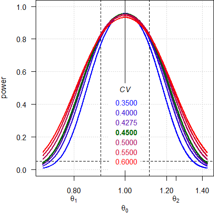
Fig. 4 Power curves for n = 28 (2×2×4 design).
Note the log-scale of the x-axis. It demonstrates that power curves are symmetrical around 1 (\(\small{\log_{e}(1)=0}\), where \(\small{\log_{e}(\theta_2)=\left|\log_{e}(\theta_1)\right|}\)) and we will achieve the same power for \(\small{\theta_0}\) and \(\small{1/\theta_0}\) (e.g., for 0.90 and 1.1111). Contrary to ABE, power is maintained.
<nitpick>-
A common flaw in protocols is the phrase
»The sample size was calculated [sic] based on a T/R-ratio of 0.90 – 1.10«
If you assume a deviation of 10% of the test from the reference and are not sure about its direction (lower or higer than 1), always use the lower T/R-ratio. If you would use the upper T/R-ratio, power would be only preserved down to 1/1.10 = 0.9091.
Given, sometimes you will need a higher sample size with the lower T/R-ratio. There’s no free lunch.
CV      <- 0.45
delta   <- 0.10 # direction unknown
design  <- "2x2x4"
theta0s <- c(1 - delta, 1 / (1 + delta),
             1 + delta, 1 / (1 - delta))
n       <- sampleN.RSABE(CV = CV, theta0 = 1 - delta,
                         design = design,
                         details = FALSE,
                         print = FALSE)[["Sample size"]]
comp1   <- data.frame(CV = CV, theta0 = theta0s,
                      base = c(TRUE, rep(FALSE, 3)),
                      n = n, power = NA)
for (i in 1:nrow(comp1)) {
  comp1$power[i] <- power.RSABE(CV = CV,
                                theta0 = comp1$theta0[i],
                                design = design, n = n)
}
n       <- sampleN.RSABE(CV = CV, theta0 = 1 + delta,
                         design = design,
                         details = FALSE,
                         print = FALSE)[["Sample size"]]
comp2   <- data.frame(CV = CV, theta0 = theta0s,
                      base = c(FALSE, FALSE, TRUE, FALSE),
                      n = n, power = NA)
for (i in 1:nrow(comp2)) {
  comp2$power[i] <- power.RSABE(CV = CV,
                                theta0 = comp2$theta0[i],
                                design = design, n = n)
}
comp1[, c(2, 5)] <- signif(comp1[, c(2, 5)] , 4)
comp2[, c(2, 5)] <- signif(comp2[, c(2, 5)] , 4)
print(comp1, row.names = FALSE)
print(comp2, row.names = FALSE)
# CV theta0 base n power
# 0.45 0.9000 TRUE 24 0.8245
# 0.45 0.9091 FALSE 24 0.8492
# 0.45 1.1000 FALSE 24 0.8499
# 0.45 1.1110 FALSE 24 0.8242
# CV theta0 base n power
# 0.45 0.9000 FALSE 22 0.7951
# 0.45 0.9091 FALSE 22 0.8199
# 0.45 1.1000 TRUE 22 0.8212
# 0.45 1.1110 FALSE 22 0.7954</nitpick>
Essentially this leads to the murky waters of prospective sensitivity
analyses, which is covered in another article.
An appetizer to show the maximum deviations (CV, T/R-ratio and
decreased sample size due to dropouts) which give still a minimum
acceptable power of ≥ 0.70:
CV       <- 0.45
theta0   <- 0.90
target   <- 0.80
minpower <- 0.70
pa       <- pa.scABE(CV = CV, theta0 = theta0,
                     targetpower = target,
                     minpower = minpower,
                     regulator = "FDA",
                     design = "2x2x4")
change.CV     <- 100*(tail(pa$paCV[["CV"]], 1) -
                      pa$plan[["CVwR"]]) /
                      pa$plan[["CVwR"]]
change.theta0 <- 100*(head(pa$paGMR$theta0, 1) -
                      pa$plan$theta0) /
                      pa$plan[["theta0"]]
change.n      <- 100*(tail(pa$paN[["N"]], 1) -
                      pa$plan[["Sample size"]]) /
                      pa$plan[["Sample size"]]
comp     <- data.frame(parameter = c("CV", "theta0", "n"),
                       change = c(change.CV,
                                  change.theta0,
                                  change.n))
comp$change <- sprintf("%+.2f%%", comp$change)
names(comp)[2] <- "relative change"
print(pa, plotit = FALSE)
print(comp, row.names = FALSE)
# Sample size plan scABE (FDA/RSABE)
# Design alpha CVwT CVwR theta0 theta1 theta2 Sample size
# 2x2x4 0.05 0.45 0.45 0.9 0.8 1.25 24
# Achieved power Target power
# 0.8245 0.8
#
# Power analysis
# CV, theta0 and number of subjects leading to min. acceptable power of ~0.7:
# CV= 1.1132, theta0= 0.8647
# n = 18 (power= 0.7141)
#
# parameter relative change
# CV +147.37%
# theta0 -3.92%
# n -25.00%Confirms what we have seen above. As expected the method is extremely robust to changes of the CV. The sample size is also not very sensitive; many overrate the impact of dropouts on power.
Heteroscedasticity
I recommend to perform pilot studies in one of the fully replicated
designs. If you are concerned about dropouts or the bioanalytical method
requires large sample volumes, opt for one the 2-sequence 3-period
designs (TRT|RTR or TRR|RTT).
Contrary to the partial replicate design (TRR|RTR|RRT) we get estimates
of both \(\small{CV_\text{wT}}\) and
\(\small{CV_\text{wR}}\). Since
pharmaceutical technology – hopefully – improves, it is not uncommon
that \(\small{CV_\text{wT}<CV_\text{wR}}\). If
this is the case, we get an incentive in the sample size of the pivotal
study (scaling is based on \(\small{CV_\text{wR}}\) but the 90%
CI on the – pooled – \(\small{s_\text{w}^{2}}\)).
\[\eqalign{\tag{7} s_\text{wT}^{2}&=\log_{e}(CV_\text{wT}^{2}+1)\\ s_\text{wR}^{2}&=\log_{e}(CV_\text{wR}^{2}+1)\\ s_\text{w}^{2}&=\left(s_\text{wT}^{2}+s_\text{wR}^{2}\right)/2\\ CV_\text{w}&=\sqrt{\exp(s_\text{w}^{2})-1}}\] It must be mentioned that \(\text{(7)}\) is only correct if the study was balanced (i.e., with an equal number of eligible subjects in each sequence). Otherwise, variances have to be weighed by the degrees of freedom.
Say, we performed two pilot studies.
In the partial replicate we estimated the \(\small{CV_\text{w}}\) with 0.45. We have to
assume homoscedasticity (\(\small{CV_\text{wT}=CV_\text{wR}}\)), which
might be wrong.
In the full replicate we estimated \(\small{CV_\text{wT}}\) with 0.414 and \(\small{CV_\text{wR}}\) with 0.484. Note
that the \(\small{CV_\text{w}}\) is
0.45 as well. How will that impact the sample size of the pivotal
4-period full replicate design?
comp <- data.frame(pilot = c("TRR|RTR|RRT", "TRT|RTR"),
                   CVwT = c(0.45, 0.414),
                   CVwR = c(0.45, 0.484),
                   CVw = NA,
                   n = NA, power = NA)
for (i in 1:nrow(comp)) {
  comp[i, 4]   <- signif(
                    mse2CV((CV2mse(comp$CVwT[i]) +
                            CV2mse(comp$CVwR[i])) / 2), 3)
  comp[i, 5:6] <- sampleN.RSABE(CV = c(comp$CVwT[i], comp$CVwR[i]),
                                 design = "2x2x4", details = FALSE,
                                 print = FALSE)[8:9]
}
print(comp, row.names = FALSE)
# pilot CVwT CVwR CVw n power
# TRR|RTR|RRT 0.450 0.450 0.45 24 0.82450
# TRT|RTR 0.414 0.484 0.45 20 0.80146Since bioanalytics drives study costs to a great extent, we may safe ~17%.
Note that when you give CV as two-element vector, the
first element has to be \(\small{CV_\text{wT}}\) and the second \(\small{CV_\text{wR}}\).
Although according to the guidances it is not required to estimate \(\small{CV_\text{wT}}\), its value is ‘nice to know’. Sometimes studies fail only due to the large \(\small{CV_\text{wR}}\) thus inflating the confidence interval. In such a case you have at least ammunation to start an argument.
Even if you plan the pivotal study in a partial replicate design (why on earth?)28 knowing both \(\small{CV_\text{wT}}\) and \(\small{CV_\text{wR}}\) is useful.
comp <- data.frame(pilot = c("TRR|RTR|RRT", "TRT|RTR"),
                   CVwT = c(0.45, 0.414),
                   CVwR = c(0.45, 0.484),
                   CVw = NA,
                   n = NA, power = NA)
for (i in 1:nrow(comp)) {
  comp[i, 4]   <- signif(
                    mse2CV((CV2mse(comp$CVwT[i]) +
                            CV2mse(comp$CVwR[i])) / 2), 3)
  comp[i, 5:6] <- sampleN.RSABE(CV = c(comp$CVwT[i], comp$CVwR[i]),
                                design = "2x3x3", details = FALSE,
                                print = FALSE)[8:9]
}
print(comp, row.names = FALSE)
# pilot CVwT CVwR CVw n power
# TRR|RTR|RRT 0.450 0.450 0.45 33 0.82802
# TRT|RTR 0.414 0.484 0.45 27 0.81239Again, a smaller sample size is possible.
Multiple Endpoints
For demonstrating bioequivalence for the FDA and China’s CDE the pharmacokinetic metrics Cmax, AUC0–t, and AUC0–∞ are mandatory.
We don’t have to worry about multiplicity issues (inflated Type I Error) since if all tests must pass at level \(\alpha\), we are protected by the intersection-union principle.29 30 We design the study always for the worst case combination, i.e., based on the PK metric requiring the largest sample size. Let’s explore that with different CVs and T/R-ratios.
metrics <- c("Cmax", "AUC")
CV      <- c(0.45, 0.30)
theta0  <- c(0.90, 0.925)
design  <- "2x2x4"
df      <- data.frame(metric = metrics, CV = CV, swR = CV2se(CV),
                      theta0 = theta0, n = NA, power = NA)
df[1, 5:6] <- sampleN.RSABE(CV = CV[1], theta0 = theta0[1],
                            design = design, details = FALSE,
                            print = FALSE)[8:9]
df[2, 5:6] <- sampleN.RSABE(CV = CV[2], theta0 = theta0[2],
                            design = design, details = FALSE,
                            print = FALSE)[8:9]
df$swR <- signif(df$swR, 5)
txt      <- paste0("Sample size based on ",
                   df$metric[df$n == max(df$n)], ".\n")
print(df, row.names = FALSE)
cat(txt)
# metric CV swR theta0 n power
# Cmax 0.45 0.42942 0.900 24 0.82450
# AUC 0.30 0.29356 0.925 22 0.81108
# Sample size based on Cmax.As usual the ‘worse’ PK metric
drives the sample size. Although we could scale for
Cmax (\(\small{s_\text{wR}\,0.42942\ge0.294}\)) but
not for AUC (\(\small{s_\text{wR}\,0.29356<0.294}\));
this advantage is counteracted by its ‘worse’ T/R-ratio (0.900 instead
of 0.925). Power is extremely sensitive to the T/R-ratio (see Fig. 4).
Consequently, with 24 subjects the study will be slightly
‘overpowered’ (~0.839) for AUC.
Let us assume the same T/R-ratios for both metrics. Which are the extreme T/R-ratios (largest deviations of T from R) for Cmax giving still the target power?
opt <- function(x) {
  power.RSABE(theta0 = x, CV = df$CV[1],
              design = design,
              n = df$n[2]) - target
}
metrics <- c("Cmax", "AUC")
CV      <- c(0.45, 0.30)
theta0  <- 0.90
target  <- 0.80
design  <- "2x2x4"
df      <- data.frame(metric = metrics, CV = CV, swR = CV2se(CV),
                      theta0 = theta0, n = NA, power = NA)
df[1, 5:6] <- sampleN.RSABE(CV = CV[1], theta0 = theta0,
                            design = design, details = FALSE,
                            print = FALSE)[8:9]
df[2, 5:6] <- sampleN.RSABE(CV = CV[2], theta0 = theta0,
                            design = design, details = FALSE,
                            print = FALSE)[8:9]
df$swR   <- signif(df$swR, 5)
df$power <- signif(df$power, 5)
if (theta0[1] < 1) {
  res <- uniroot(opt, tol = 1e-8,
                 interval = c(0.80 + 1e-4, theta0))
} else {
  res <- uniroot(opt, tol = 1e-8,
                 interval = c(theta0, 1.25 - 1e-4))
}
res     <- unlist(res)
theta0s <- c(res[["root"]], 1/res[["root"]])
txt     <- paste0("Target power for ", metrics[1],
                  " and sample size ",
                  df$n[2], "\nachieved for theta0 ",
                  sprintf("%.4f", theta0s[1]), " or ",
                  sprintf("%.4f", theta0s[2]), ".\n")
print(df, row.names = FALSE)
cat(txt)
# metric CV swR theta0 n power
# Cmax 0.45 0.42942 0.9 24 0.82450
# AUC 0.30 0.29356 0.9 32 0.81666
# Target power for Cmax and sample size 32
# achieved for theta0 0.8661 or 1.1546.That means, although we assumed for Cmax the same T/R-ratio as for AUC, with the sample size of 32 required AUC, for Cmax it can be as low as ~0.866 or as high as ~1.155, which is an interesting side-effect.
Q & A
Q: Can we use R in a regulated environment and is
PowerTOSTvalidated?
A: See this document31 about the acceptability of BaseRand its SDLC.32
Ris updated every couple of months with documented changes33 and maintaining a bug-tracking system.34 I recommed to use always the latest release.
The authors ofPowerTOSTtried to do their best to provide reliable and valid results. Its ‘NEWS’ documents the development of the package, bug-fixes, and introduction of new methods. Issues are tracked at GitHub (as of today none is still open). So far the package had >100,000 downloads. Therefore, it is extremely unlikely that bugs were not detected given its large user base.
Validation of any software (yes, of SAS as well…) lies in the hands of the user.35 36
Execute the scripttest_RSABE.Rin the/testssub-directory of the package to reproduce tables given in the literature.37 You will notice some discrepancies: The authors employed only 10,000 simulations – which is not sufficient for a stable result (see below). Furthermore, they reported the minimum sample size which gives at least the target power, wherassampleN.RSABE()always rounds up to obtain balanced sequences.Q: Shall we throw away our sample size tables?
A: Not at all. File them in your archives to collect dust. Maybe in the future you will be asked by an agency how you arrived at a sample size. But: Don’t use them any more. What you should not do (and hopefully haven’t done before): Interpolate. Power and therefore, the sample size depends in a highly nonlinear fashion on the five conditions listed above, which makes interpolation of values given in table a nontrivial job.Q: I fail to understand your example about dropouts. We finish the study with 24 eligible subjects as desired. Why is the dropout-rate ~20% and not the anticipated 15%?
A: That’s due to rounding up the calculated adjusted sample size (28.24…) to the next even number (30). If you manage it to dose fractional subjects (I can’t), your dropout rate would indeed equal the anticipated one: 100 × (1 – 24/28.24…) = 15%. ⬜Q: Do we have to worry about unbalanced sequences?
A:sampleN.RSABE()will always give the total number of subjects for balanced sequences.
If you are interested in post hoc power, give the sample size as a vector, i.e.,power.RSABE(..., n = c(foo, bar, baz), wherefoo,bar, andbazare the number of subjects per sequence.Q: The default number of simulations in the sample size estimation is 100,000. Why?
A: We found that with this number the simulations are stable. For the background see another article. Of course, you can give a larger number in the argumentnsims. However, you shouldn’t decrease the number.
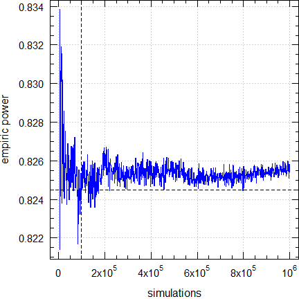
Fig. 5 Empiric power for n
= 24 (2×2×4 design).
Dashed lines give the result (0.8245) obtained
by the default (100,00 simulations).
Q: How reliable are the results?
A: As stated above an exact method doesn’t exist. We can only compare the empiric power of the ABE-component to the exact one obtained bypower.TOST(). For an example see ‘Post hoc Power’ in the section about Dropouts.Q: I still have questions. How to proceed?
A: The preferred method is to register at the BEBA Forum and post your question in the category or (please read the Forum’s Policy first).
You can contact me at [email protected]. Be warned – I will charge you for anything beyond most basic questions.
Licenses
 Helmut Schütz 2023
R and PowerTOST GPL 3.0,
klippy MIT,
pandoc GPL 2.0.
1st version March 27, 2021. Rendered June 21, 2023 10:54 CEST
by rmarkdown
via pandoc in 0.91 seconds.
Footnotes and References
Labes D, Schütz H, Lang B. PowerTOST: Power and Sample Size for (Bio)Equivalence Studies. Package version 1.5.4.9000. 2022-04-25. CRAN.↩︎
Schütz H. Reference-Scaled Average Bioequivalence. 2022-02-19. CRAN.↩︎
Labes D, Schütz H, Lang B. Package ‘PowerTOST’. February 19, 2022. CRAN.↩︎
Some gastric resistant formulations of diclofenac are HVDPs, practically all topical formulations are HVDPs, whereas diclofenac itself is not a HVD (\(\small{CV_\text{w}}\) of a solution ~8%).↩︎
Tóthfalusi L, Endrényi L, Midha KK, Rawson MJ, Hubbard JW. Evaluation of the Bioequivalence of Highly-Variable Drugs and Drug Products. Pharm Res. 2001; 18(6): 728–33. doi:10.1023/a:1011015924429.↩︎
Tóthfalusi L, Endrényi L, García-Arieta A. Evaluation of bioequivalence for highly variable drugs with scaled average bioequivalence. Clin Pharmacokinet. 2009; 48(11): 725–43. doi:10.2165/11318040-000000000-00000.↩︎
FDA, CDER. Draft Guidance for Industry. Bioequivalence Studies with Pharmacokinetic Endpoints for Drugs Submitted Under an ANDA. Silver Spring. August 2021. Download.↩︎
FDA, CDER. Draft Guidance for Industry. Statistical Approaches to Establishing Bioequivalence. Revision 1. Silver Spring. December 2022. Download.↩︎
CDE. Annex 2. Technical guidelines for research on bioequivalence of highly variable drugs. Download. [Chinese].↩︎
For unfathomable reasons the FDA recommends a mixed-effects model for fully replicated designs (SAS PROC MIXED) and a fixed-effects model (SAS PROC GLM) for the partial replicate design.↩︎
Schuirmann D. U.S. FDA Perspective: Statistical Aspects of OGD’s Approach to Bioequivalence (BE) Assessment for Highly Variable Drugs. Presentation at the 2nd conference of The Global Harmonisation Initiative (GBHI). Rockville. September 15–16, 2016.↩︎
Howe WG. Approximate Confidence Limits on the Mean of X+Y Where X and Y are Two Tabled Independent Random Variables. J Am Stat Assoc. 1974; 69(347): 789–94. doi:10.2307/2286019.↩︎
Davit BM, Chen ML, Conner DP, Haidar SH, Kim S, Lee CH, Lionberger RA, Makhlouf FT, Nwakama PE, Patel DT, Schuirmann DJ, Yu LX. Implementation of a Reference-Scaled Average Bioequivalence Approach for Highly Variable Generic Drug Products by the US Food and Drug Administration. AAPS J. 2012; 14(4): 915–24. doi:10.1208/s12248-012-9406-x.
 Free
Full Text.↩︎
Free
Full Text.↩︎At a \(\small{CV_{\text{wR}}}\) which is infinitesimally lower than \(\small{CV_{\text{wR}}\;0.30047}\) the ‘implied limits’ are still 80.00 – 125.00% but ‘jump’ to 76.92 – 130.01% at \(\small{CV_{\text{wR}}\approx0.30047}\).↩︎
That’s contrary to ABE, where \(\small{CV_\text{w}}\) is an assumption as well.↩︎
Senn S. Guernsey McPearson’s Drug Development Dictionary. 21 April 2020. Online.↩︎
Hoenig JM, Heisey DM. The Abuse of Power: The Pervasive Fallacy of Power Calculations for Data Analysis. Am Stat. 2001; 55(1): 19–24. doi:10.1198/000313001300339897.
 Open
Access.↩︎
Open
Access.↩︎There is no statistical method to ‘correct’ for unequal carryover. It can only be avoided by design, i.e., by a sufficiently long washout between periods. According to the guidelines subjects with pre-dose concentrations > 5% of their Cmax can by excluded from the comparison if stated in the protocol.↩︎
This is not always the case in RSABE. This issue is elaborated in another article.↩︎
Senn S. Statistical Issues in Drug Development. Chichester: John Wiley; 2nd ed 2007.↩︎
Zhang P. A Simple Formula for Sample Size Calculation in Equivalence Studies. J Biopharm Stat. 2003; 13(3): 529–38. doi:10.1081/BIP-120022772.↩︎
Don’t be tempted to give a ‘better’ T/R-ratio – even if based on a pilot or a previous study. It is a natural property of HVD(P)s that the T/R-ratio varies between studies. Don’t be overly optimistic!↩︎
Doyle AC. The Adventures of Sherlock Holmes. A Scandal in Bohemia. 1892. p. 3.↩︎
Schütz H. Sample Size Estimation in Bioequivalence. Evaluation. 2020-10-23. BEBA Forum.↩︎
Lenth RV. Two Sample-Size Practices that I Don’t Recommend. October 24, 2000. Online.↩︎
The only exception is
design = "2x2x3"(the full replicate with sequences TRT|RTR). Then the first element is for sequence TRT and the second for RTR.↩︎Quoting my late father: »If you believe, go to church.«↩︎
For obstacles see this article.↩︎
Berger RL, Hsu JC. Bioequivalence Trials, Intersection-Union Tests and Equivalence Confidence Sets. Stat Sci. 1996; 11(4): 283–302. JSTOR:2246021.↩︎
Zeng A. The TOST confidence intervals and the coverage probabilities with R simulation. March 14, 2014. Online.↩︎
The R Foundation for Statistical Computing. A Guidance Document for the Use of R in Regulated Clinical Trial Environments. Vienna. October 18, 2021. Online.↩︎
The R Foundation for Statistical Computing. R: Software Development Life Cycle. A Description of R’s Development, Testing, Release and Maintenance Processes. Vienna. October 18, 2021. Online.↩︎
FDA. Statistical Software Clarifying Statement. May 6, 2015. Online.↩︎
WHO. Guidance for organizations performing in vivo bioequivalence studies. Geneva. May 2016. Technical Report Series No. 996, Annex 9. Section 4. Online.↩︎
Tóthfalusi L, Endrényi L. Sample Sizes for Designing Bioequivalence Studies for Highly Variable Drugs. J Pharm Pharmaceut Sci. 2012; 15(1): 73–84. doi:10.18433/J3Z88F.
Open
Access.↩︎