
Demonstration of Steady State Achievement?
Helmut Schütz

March 13, 2025
Consider allowing JavaScript. Otherwise, you have to be proficient in
reading  since formulas
will not be rendered. Furthermore, the table of contents in the left
column for navigation will not be available and code-folding not
supported. Sorry for the inconvenience.
since formulas
will not be rendered. Furthermore, the table of contents in the left
column for navigation will not be available and code-folding not
supported. Sorry for the inconvenience.
Scripts were run on a Xeon E3-1245v3 @ 3.40GHz (1/4 cores) 16GB RAM
with
 4.4.3 on Windows 7 build 7601, Service Pack 1, Universal C Runtime
10.0.10240.16390.
4.4.3 on Windows 7 build 7601, Service Pack 1, Universal C Runtime
10.0.10240.16390.
The right-hand badges give the respective section’s ‘level’.
- Basics about Pharmacokinetics (PK) – requiring no or only limited expertise.
- The most important sections. They are – hopefully – easily comprehensible even for novices.
- A higher knowledge of PK and/or R is required. Sorry, there is no free lunch.
- An advanced knowledge of PK and/or R is required. Not recommended for beginners in particular.
- If you are not a neRd or PK afficionado, skipping is recommended. Suggested for experts but might be confusing for others.
- Click to show / hide R code.
- To copy R code to the clipboard click on
the icon
 in the top left corner.
Introduction
Which method should we use to demonstrate achievement of steady state?
First of all, design the study based on a worst-case half
life (not an average).
Especially for prolonged (aka
controlled, sustained, extended, long-acting) release formulations
consider flip-flop Pharmacokinetics.
“You can’t fix by analysis what you bungled by design.
Background
For a comparative bioavailability study we have essentially two design options:
- Single dose
- Multiple dose
The former is recommended in all guidelines for comparing immediate release formulations because it is more sensitive in detecting potential differences in formulations (especially of the rate of absorption \(\small{C_\textrm{max}}\) / \(\small{t_\textrm{max}}\)). Only in rare cases (e.g., an auto-inducer like carbamazepine4) studies after multiple doses are more sensitive than after a single dose.
The latter is required in studies in patients, where the treatment cannot be interrupted with washout phases (e.g., in oncology). It is mandatory for the EMA when comparing prolonged release formulations – additionally to the single dose study.
“Steady-state, the condition in which the amount lost from the body during a dosing interval equals the amount input on a regimen of fixed dose and dosing interval is, in theory approached but never achieved. The question is how close one must be to declare practical achievement of steady-state. From a clinical perspective, 90% of the theoretic steady-state value is often used as a practical definition, as the difference in response to a 10% difference in concentration can rarely be assessed […] although other choices of a percentage are possible.
Guidelines
Past
“In steady-state studies, wash-out of the last dose of the previous treatment can overlap with the build-up of the second treatment, provided the build-up period is sufficiently long (at least three times the dominating half-life).
“Whenever multiple dose studies are performed it should be demonstrated that steady state has been reached.
“In steady-state studies wash out of the previous treatment last dose can overlap with the build-up of the second treatment, provided the build-up period is sufficiently long (at least three times the terminal half-life).
A similar wording is used by the WHO,9 only that »at least five times the terminal half-life« are recommended.
In Europe regularly a linear regression of the last three pre-dose concentrations was performed, allowing to exclude subjects who are not in steady state. The idea behind is based on elementary pharmacokinetics. By definition in steady state inflow equals outflow. Hence, in all dosing intervals the pre-dose concentrations (\(\small{C_{\textrm{pd}}}\)) are expected to be similar. Therefore, a linear regression should give a slope close to zero. However, this approach was based on custom and not backed by a guideline.
Recall the ‘Accumulation Index’ \(\small{R=1/(1-2^{-\tau\,/\,t_{1/2}}\,)}\).
\(\small{R}\) is strictly valid for
intravenous doses and approximate for extravascular administrations in a
one-compartment model if \(\small{k_{01}\gg
k_{10}}\).
An example with \(\small{\tau=t_{1/2}\;(R=2)}\), where \(\small{C_\textrm{pd}}\) is the pre-dose
concentration and \(\small{C_\tau}\) is
the concentration at the end of the dosing interval. Values ‘by
definition’ are denoted with \(\small{\ast}\). \[\small{
\begin{array}{rrrrrr}
\text{dose} & \text{time} & C_\textrm{pd}\phantom{00000} &
\text{% change} & \text{moving slope} & C_\tau\phantom{000000}\\
\hline
1 & 0 & 0\phantom{.000000}\phantom{0} & - & - &
50\phantom{.00000000}\\
2 & 24 & 50\phantom{.0000000} & 50\phantom{.0000000} & -
& 75\phantom{.00000000}\\
3 & 48 & 75\phantom{.0000000} & 16.6666667 & 0.78125
& 87.5\phantom{0000000}\\
4 & 72 & 87.5\phantom{000000} & 7.1428571 & 0.39063
& 93.75\phantom{000000}\\
5 & 96 & 93.75\phantom{00000} & 3.3333333 & 0.19531
& 96.875\phantom{00000}\\
6 & 120 & 96.875\phantom{0000} & 1.6129032 & 0.09766
& 98.4375\phantom{0000}\\
7 & 144 & 98.4375\phantom{000} & 0.7936508 & 0.04883
& 99.21875\phantom{000}\\
8 & 168 & 99.21875\phantom{00} & 0.3937008 & 0.02441
& 99.609375\phantom{00}\\
9 & 192 & 99.609375\phantom{0} & 0.1960784 & 0.01221
& 99.8046875\phantom{0}\\
10 & 216 & 99.8046875 & 0.0978474 & 0.00610 &
99.90234375\\
\infty & \infty & 100\phantom{.0000000} &
0\ast\phantom{.00000} & 0\ast\phantom{.000} &
100\;(=C_\textrm{pd})\phantom{0}\\
\hline
\end{array}}\]
Health Canada required 1992 – 2011 multiple dose studies for drugs which accumulated, i.e., if the extrapolated \(\small{AUC}\) after a single dose was > 20% of \(\small{AUC_{0-\infty}}\).
“7.6.2 Evidence of Steady State
For steady-state studies of drugs with uncomplicated characteristics, at least three consecutive pre-dose concentration levels (Cpd) are required to provide evidence of steady state. Generally, observations of Cpd for the test and reference products should be recorded at the same time of the day. One of these measurements could be taken based on the first sample of the study day in which a profile over the dosing interval is being established. Steady state is usually achieved when repeated doses of a formulation are administered over a period that exceeds five disposition half-lives of the modified-release form.
‘Evidence of steady state’ had to be assessed by a repeated measures analysis with an amazing number of 11 (eleven‼) factors. If you want to give it a try, download the data compiled from the guidance’s Table 12-A (Randomization), Table 12-G (Test), and Table 12-H (Reference).
data     <- read.csv("https://bebac.at/downloads/HC1996-TABLE-12.csv",
                     colClasses = c(rep("factor", 5), "integer"))
geo.mean <- function(x) {
  t  <- as.numeric(unlist(unique(x[1])))
  n  <- as.integer(unlist(unique(x[2])))
  gm <- NA_real_
  for (i in seq_along(t)) {
    y <- x[x[1] == t[i], ]
    if (sum(y$C <= 0) > 0) {
      y <- y[-which(y$C <= 0), ]
    }
    if (nrow(y) > 0) {
      gm[i] <- exp(mean(log(y$C), na.rm = TRUE))
    }
  }
  return(gm)
}
Subject <- unique(as.character(data$Subject))
Form    <- unique(as.character(data$Formulation))
slopes  <- data.frame(Formulation = rep(Form, each = length(Subject)),
                      Subject = Subject, slope = NA_real_,
                      lower.CL = NA_real_, upper.CL = NA_real_,
                      sig = FALSE)
t       <- data$Time
t       <- as.numeric(levels(t))[t]
ylim    <- range(data$C.pd)
xlim    <- range(t)
cols    <- c("blue", "red")
col     <- colorRampPalette(cols)(length(Subject))
col     <- paste0(col, "80")
op      <- par(no.readonly=TRUE)
par(mar = c(4.1, 4, 0.2, 0.2), cex.axis = 0.9)
split.screen(c(2, 1))
for (i in seq_along(Form)) {
  screen(i)
  ifelse (i == 1, xlab  <- "", xlab <- "Time (day)")
  plot(xlim, ylim, type = "n", las = 1, xlab = xlab,
       ylab = paste0("C.pd  (", Form[i], ")"))
  grid()
  x <- data.frame(t = t,
                  C = data[data$Formulation == Form[i], 6])
  lines(unique(t), geo.mean(x), lwd = 2)
  for (j in seq_along(Subject)) {
    t  <- data$Time[data$Formulation == Form[i] &
                    data$Subject == Subject[j]]
    t  <- as.numeric(levels(t))[t]
    C  <- data$C.pd[data$Formulation == Form[i] &
                    data$Subject == Subject[j]]
    points(t, C, pch = 16, cex = 1.1, col = col[j])
    x  <- data.frame(t = t, C = C)
    x  <- tail(x, 3)
    m  <- lm(C ~ t, data = x)
    lines(x$t, predict(m), col = substr(col[j], 1, 7))
    slopes$slope[slopes$Formulation == Form[i] &
                 slopes$Subject == Subject[j]] <- coef(m)[2]
    ci <- suppressWarnings(confint(m, "t"))
    slopes[slopes$Formulation == Form[i] &
           slopes$Subject == Subject[j], 4:5] <- sprintf("%+.4f", ci)
    if (sign(ci[1]) == sign(ci[2]))
      slopes$sig[slopes$Formulation == Form[i] &
                 slopes$Subject == Subject[j]] <- TRUE
  }
}
close.screen(all = TRUE)
par(op)
slopes$slope     <- sprintf("%+5.1f", slopes$slope)
names(slopes)[6] <- "sign # 0"
last.3 <- data[as.numeric(as.character(data$Time)) >= 6, ]
muddle <- lm(log(C.pd) ~ Sequence + Subject * Sequence + Period +
                         Formulation + Subject * Formulation * Sequence +
                         Time + Time * Sequence + Time * Subject * Sequence +
                         Time * Period + Time * Period +
                         Time * Formulation * Subject * Sequence,
                         data = last.3)
print(slopes, row.names = FALSE); anova(muddle) # Oops!“Of main importance in this analysis is the time and time*form interaction. The error term to test time is the time*ID(Seq). The error term to test time*form is time*form*ID(Seq). Should either the time or time*form effects be significant, the study may not have been at steady state for one or both formulations.
Back in the day I failed to reproduce the results given in Table 12-I.
In R I got …
Analysis of Variance Table
Response: log(C.pd)
                         Df  Sum Sq  Mean Sq F value Pr(>F)
Sequence                  1 0.01326 0.013260     NaN    NaN
Subject                  10 1.22059 0.122059     NaN    NaN
Period                    1 0.01825 0.018249     NaN    NaN
Formulation               1 0.22069 0.220686     NaN    NaN
Time                      2 0.11935 0.059675     NaN    NaN
Subject:Formulation      10 0.56173 0.056173     NaN    NaN
Sequence:Time             2 0.13041 0.065204     NaN    NaN
Subject:Time             20 0.71386 0.035693     NaN    NaN
Period:Time               2 0.06441 0.032204     NaN    NaN
Formulation:Time          2 0.05961 0.029804     NaN    NaN
Subject:Formulation:Time 20 0.60824 0.030412     NaN    NaN
Residuals                 0 0.00000      NaN
Warning message:
In anova.lm(m) : ANOVA F-tests on an essentially perfect fit are unreliable
… and in Phoenix WinNonlin (all effects fixed):
ERROR 11068: There are no degrees of freedom for residual. No tests are possible.When I specified all subject-related effects as random:
      Hypothesis  Numer_DF  Denom_DF    F_stat      P_value
–––––––––––––––––––––––––––––––––––––––––––––––––––––––––––
             int         1        60   4446.56       0.0000
        Sequence         1        60      0.0609162  0.8059
     Formulation         1        60      3.04158    0.0863
            Time         2        60      1.00778    0.3711
   Time*Sequence         2        60      1.19822    0.3088
     Time*Period         3        60      1.59434    0.2002
Time*Formulation         2        60      1.64308    0.2020
\[\small{\text{TABLE 12-I }\textsf{(in all of its doubtful beauty)}}\] \[\small{\begin{array}{lrcccc} \hline\text{Source} & \text{df} & \text{SS} & \text{MS} & \text{F} & \text{PR > F}\\\hline \text{Seq} & 1 & 0.01500416 & 0.01500416 & 0.12 & 0.7313\\ \text{ID(Seq)} & 10 & 1.20256303 & 1.20256303 & 2.11 & 0.1278\\ \text{Period} & 1 & 0.04556284 & 0.04556284 & 0.80 & 0.3926\\ \text{Form} & 1 & 0.22620312 & 0.22620312 & 3.96 & 0.0745\\ \text{ID*Form(Seq)} & 10 & 0.57066567 & 0.0570666\phantom{0} & - & -\\ \text{Time} & 2 & 0.11182757 & 0.05591378 & 1.60 & 0.2274\\ \text{Time*Seq} & 10 & 0.13927056 & 0.06963528 & 1.99 & 0.1631\\ \text{Time*ID(Seq)} & 20 & 0.70058566 & 0.03502928 & - & -\\ \text{Time*Period} & 2 & 0.07672565 & 0.03836282 & 1.24 & 0.3110\\ \text{Time*Form} & 2 & 0.06390201 & 0.03195101 & 1.03 & 0.3746\\ \text{Time*Form*ID(Seq)} & 20 & 0.61937447 & 0.03096872 & - & -\\ \text{Corrected Total} & 71 & 3.74093818 & - & - & -\\\hline \end{array}}\] Maybe you are equipped with Harry Potter’s magic wand. If you succeed in reproducing this table, drop me a note how you did it. I’m always eager to learn.
However, the outcome of such an analysis is dichotomous (pass |
fail), risking to discard the entire [sic] study. The family-wise
error rate of two simultaneous tests (here \(\small{\text{Time}}\) and \(\small{\text{Time*Form}}\)) at level \(\small{\alpha}\) is given by \[FWER=1-(1-\alpha)^2
\tag{1}\] or 9.75% for \(\small{\alpha=0.05}\). That means,
following this method you may have to trash almost one of ten studies
although steady state was achieved.
Given, that is only of historical interest.
Current
“Achievement of steady state can be evaluated by collecting pre-dose samples on the day before the PK assessment day and on the PK assessment day. A specific statistical method to assure that steady state has been reached is not considered necessary in bioequivalence studies. Descriptive data is sufficient.
Two pre-dose samples, right? Interesting.
The requirement of performing multiple dose studies was lifted by Health Canada in 2012. However, if such studies are performed, the pre-dose concentrations determined immediately before a dose at steady state (Cpd) have to be reported.12
“Because single-dose studies are considered more sensitive in addressing the primary question of BE (e.g., release of the drug substance from the drug product into the systemic circulation), multiple-dose studies are generally not recommended.
A statistical method is not given in any guidance of the FDA. A statement about the current practice:14
“Current FDA practice for general procedure for steady-state assessment is by comparing at least three pre-dose concentrations for each formulation using linear regression techniques to evaluate achievement of steady state and by comparing the BE outcome with or without the subjects whose terminal slope is significantly different from 0 (i.e., they did not attain steady state).
“Whenever multiple dose studies are performed it should be demonstrated that steady state has been reached. Achievement of steady-state is assessed by comparing at least three pre-dose concentrations for each formulation, unless otherwise justified.
Wait a minute! A breakdown by formulation and not by subject? Which values are we supposed to use? Geometric or arithmetic means, medians?
Since the EMA’s guideline is adopted in Australia, the same story Down Under.16
Even less details are given by the ICH.17
“[…] applicants should document appropriate dosage administration and sampling to demonstrate the attainment of steady-state. For steady-state studies, the following PK parameters should be tabulated: 1) primary parameters for analysis: CmaxSS and AUC(0-tauSS), and 2) additional parameters for analysis: CtauSS, CminSS, CavSS, degree of fluctuation, swing, and Tmax.
No details are given by the ANVISA as well.18
“Devendo ser assegurada a obtenção do estado de equilíbrio antes das coletas das amostras.
Em estudos com doses múltiplas, a amostra pré-dose deve ser coletada imediatamente antes da última administração da medicação.
[It must be ensured that equilibrium state is reached before the samples are taken.
In multiple dose studies, the pre-dose sample should be collected immediately prior to the last drug administration.]
Regression Analyses
While appealing,19 20 a regression approach is problematic.
- In any regression it is assumed that responses are not correlated (i.e., depend only on the predictor). In PK clearly this is not the case – pre-dose concentrations are highly correlated. Perform a Durbin–Watson test – you will be surprised.
- The outcome depends on the within-subject variability:
- If it is low to intermediate, it is quite likely that some subjects
show a slope which is statistically significant different from zero (or
alternatively, its confidence interval (CI) does not contain
zero).
It will be – falsely – concluded that the respective subjects are not in steady-state. - If it is high, a significant difference of the slope to zero
(i.e., the CI contains
zero) will not be detected – although some subjects are still in the
build-up / saturation phase.
It will be – falsely – concluded that steady-state is achieved.
- If it is low to intermediate, it is quite likely that some subjects
show a slope which is statistically significant different from zero (or
alternatively, its confidence interval (CI) does not contain
zero).
Linear model
For every subject a linear model is set up \[Y=a+bX+\epsilon\small{\textsf{,}}\tag{2}\] where \(\small{Y}\) is the vector of responses (here at least three pre-dose concentrations), \(\small{X}\) the vector of predictors (the corresponding sampling time points), and \(\epsilon\) the unexplained error with \(\small{\mathcal{N}(0;\sigma^2)}\). Fitting the data gives estimates of the intercept \(\small{\hat{a}}\) and slope \(\small{\hat{b}}\). One can either perform a one-sample t-test of \(\small{\hat{b}}\) versus zero with \(\small{\alpha=0.05}\) (significantly different if \(\small{p(\hat{b})<0.05}\)) or assess whether zero is contained in the 95% CI of \(\small{\hat{b}}\). Since the latter is more ‘popular’, we employed it in the following.
The script is for a one-compartment model, first order absorption and elimination with an optional lag-time. Flip-flop PK (\(\small{k_{01}=k_{10}}\)) is implemented. Cave: 288 LOC.
sim.ss <- function(nsims, f, D, V, t12.a, t12.e, tlag, tau, fact,
                   CV.lo = 0.1, CV.hi = 0.4, delta = 0.2,
                   method = "linear", dw = FALSE, setseed = TRUE,
                   progress = FALSE, plots = FALSE) {
  suppressMessages(library(car)) # for Durbin-Watson
  # Cave: Long run time if nsims > 1e4
  #       Extremely long run time if dw = TRUE
  if (nsims < 1)      stop("nsims must be at least 1.")
  if (f <= 0 | f > 1) stop("f must be positive and <= 1.")
  if (D <= 0)         stop("D must be positive.")
  if (t12.a <= 0)     stop("t12.a (absorption half life) must be positive.")
  if (t12.e <= 0)     stop("t12.e (elimination half life) must be positive.")
  if (tlag < 0)       stop("tlag must >= 0.")
  if (tau < 0)        stop("tau must be positive.")
  if (CV.lo <= 0)     stop("CV.lo must be positive.")
  if (CV.hi <= 0)     stop("CV.hi must be positive.")
  if (delta < 0)      stop("delta must be positive.")
  if (fact < 3) {
    message("fact < 3 not reasonable. Forced to 3.")
    fact <- 3
  }
  if (!method %in% c("linear", "power")) stop("method not supported.")

  one.comp <- function(f, D, V, k01, k10, tlag, t) {
    # one-compartment model, first order absorption
    # and elimination
    if (!isTRUE(all.equal(k01, k10))) {# common: k01 != k10
      C    <- f * D * k01 / (V * (k01 - k10)) *
              (exp(-k10 * (t - tlag)) - exp(-k01 * (t - tlag)))
      tmax <- log(k01 / k10) / (k01 - k10) + tlag
      Cmax <- f * D * k01 / (V * (k01 - k10)) *
              (exp(-k10 * tmax) - exp(-k01 * tmax))
    } else {                           # flip-flop
      k    <- k10
      C    <- f * D / V * k * (t - tlag) * exp(-k * (t - tlag))
      tmax <- 1 / k
      Cmax <- f * D / V * k * tmax * exp(-k * tmax)
    }
    C[C <= 0] <- 0 # correct negatives caused by lag-time
    res <- list(C = C, Cmax = Cmax, tmax = tmax)
    return(res)
  }

  round.up <- function(x, y) {
    # round x up to the next multiple of y
    return(as.integer(y * (x %/% y + as.logical(x %% y))))
  }

  superposition <- function(f, D, V, k01, k10, tlag, tau, t, n.D) {
    # single dose
    x         <- data.frame(adm = 1L, dose = NA, t = t,
                            C = one.comp(f, D, V, k01, k10, tlag, t)$C)
    x$dose[1] <- D
    # multiple dose (nonparametric superposition)
    y <- x
    for (i in 1:nrow(y)) {
      if (isTRUE(all.equal(y$t[i] %% tau, 0))) y$dose[i] <- D
    }
    delta <- unique(diff(y$t))
    adm   <- seq(0, max(y$t), tau) # administration times
    adm.n <- 1:length(adm)         # number of administration
    if (isTRUE(all.equal(delta, tau))) {# for pre-dose concentrations
      y$adm <- adm.n
    } else {                            # for build-up
      t.tau <- sum(y$t < tau)
      y$adm <- head(rep(adm.n, each = t.tau), nrow(y))
    }
    z <- 2:(n.D + 1)
    for (i in seq_along(z)) {
      tmp.y              <- y$C[y$adm >= z[i]]
      tmp.x              <- x$C[1:length(tmp.y)]
      y$C[y$adm >= z[i]] <- tmp.y + tmp.x
    }
    res <- list(SD = x, MD = y)
    return(res)
  }

  CV2var <- function(CV) {
    # convert CV to variance
    return(log(CV^2 + 1))
  }

  mods <- function(x, method = "linear", dw = FALSE, delta = 0.2) {
    # last three pre-dose concentrations
    x <- tail(x, 3)
    # model and 95% CI of slope
    if (method == "linear") {
      m  <- lm(C ~ t, data = x)
      a  <- coef(m)[[1]]
      ci <- confint(m, "t", level = 0.95)
      if (dw) dw.p <- dwt(m, reps = 1e4)$p
    }
    if (method == "power") {
      m  <- lm(log(C) ~ log(t), data = x)
      a  <- exp(coef(m)[[1]])
      ci <- confint(m, "log(t)", level = 0.95)
      if (dw) dw.p <- dwt(m, reps = 1e4)$p
    }
    # assess whether the CI contains zero
    ifelse (sign(ci[1]) == sign(ci[2]), sig1 <- TRUE, sig1 <- FALSE)
    # assess whether the CI is within +/- delta
    ifelse ((ci[1] >= -delta & ci[2] <= +delta), sig2 <- FALSE, sig2 <- TRUE)
    res <- list(method = method, a = a, b = coef(m)[[2]],
                lwr = ci[[1]], upr = ci[[2]], sig1 = sig1, sig2 = sig2,
                t.start = x$t[1], t.end = x$t[3], dw.p = dw.p)
    return(res)
  }

  geo.mean <- function(x) {
    # geometric mean
    n <- as.integer(unlist(unique(x[1])))
    t <- as.numeric(unlist(unique(x[2])))
    gm <- NA_real_
    for (i in seq_along(t)) {
      y <- x[x[2] == t[i], ]
      if (sum(y$C <= 0) > 0) {
        y <- y[-which(y$C <= 0), ] # only positive values
      }
      if (nrow(y) > 0) {
        gm[i] <- exp(mean(log(y$C), na.rm = TRUE))
      }
    }
    return(gm)
  }

  if (nsims > 1e4) progress <- TRUE  # to keep the spirit high
  k01    <- log(2) / t12.a           # absorption rate constant
  k10    <- log(2) / t12.e           # elimination rate constant
  ifelse (t12.e >= t12.a, t.last <- fact * t12.e, t.last <- fact * t12.a)
  t.last <- round.up(t.last, tau)    # time of last dose
  t      <- seq(0, t.last, tau)      # time of administrations
  n.D    <- length(t)                # number of doses
  if (setseed) set.seed(1234567)     # for reproducibility
  # build-up (high resolution)
  t.bu     <- seq(0, t.last, length.out = (t.last * 10 + 1))
  bu       <- superposition(f, D, V, k01, k10, tlag, tau, t = t.bu, n.D)$MD
  # pre-dose concentrations
  MD       <- bu[!is.na(bu$dose), ]
  mod.a    <- mods(MD, method, dw)$a # intercept without error
  mod.b    <- mods(MD, method, dw)$b # slope/exponent without error
  C.ss     <- tail(MD$C, 1)          # last pre-dose of model
  # simulated pre-dose concentrations
  sim.lo   <- sim.hi <- data.frame(sim = rep(1:nsims, each = n.D),
                                   t = t, C = NA_real_)
  # results with low and high variability
  lo       <- hi <- data.frame(sim = 1:nsims, method = NA_character_,
                               a = NA_real_, b = NA_real_,
                               lwr = NA_real_, upr = NA_real_,
                               sig1 = NA, sig2 = NA,
                               t.start = NA_real_, t.end = NA_real_)
  if (progress) pb <- txtProgressBar(0, 1, 0, char = "\u2588",
                                     width = NA, style = 3)
  for (sim in 1:nsims) {
    # multiplicative error
    C.lo <- rlnorm(n       = n.D,
                   meanlog = log(MD$C) - 0.5 * CV2var(CV.lo),
                   sdlog   = sqrt(CV2var(CV.lo)))
    C.hi <- rlnorm(n       = n.D,
                   meanlog = log(MD$C) - 0.5 * CV2var(CV.hi),
                   sdlog   = sqrt(CV2var(CV.hi)))
    sim.lo$C[sim.lo$sim == sim] <- C.lo
    sim.hi$C[sim.hi$sim == sim] <- C.hi
    # get slope, 95% CI, and significance
    lo[sim, 2:11] <- mods(sim.lo[sim.lo$sim == sim, ], method, dw)
    hi[sim, 2:11] <- mods(sim.hi[sim.lo$sim == sim, ], method, dw)
    if (progress) setTxtProgressBar(pb, sim / nsims)
  } # simulations running...
  if (progress) close(pb)
  if (method == "linear") {
    txt <- "slope"
    me  <- "linear model: C ~ a + b * t"
 } else {
    txt <- "exponent"
    me  <- "power model: C ~ a * t^b"
  }
  me <- paste(me, "\n delta =", delta,
              "(acceptance limits {-delta, +delta})\n")
  # cosmetics
  fm <- paste0("CV = %4.1f%%, median of ", txt, "s = %+.5f")
  fm <- paste0(fm, "\n  %5.1f%% positive ", txt, "s")
  fm <- paste0(fm, "\n  %5.1f%% negative ", txt, "s")
  fm <- paste0(fm, "\n   significant ", txt, "s: %6.2f%% %s")
  fm <- paste0(fm, "\n   failed ", txt, "s     : %6.2f%% %s")
  # results
  txt <- paste(prettyNum(nsims, format = "d", big.mark =","), "simulations,",
               me, txt, "of model =", sprintf("%+.5f", mod.b),
               "\n last model’s pre-dose concentration =", signif(C.ss, 4), "\n",
               sprintf(fm, 100 * CV.lo, median(lo$b),
                       100 * sum(lo$b > 0) / nsims,
                       100 * sum(lo$b < 0) / nsims,
                       100 * sum(lo$sig1, na.rm = TRUE) / nsims,
                       "(95% CI does not contain zero)",
                       100 * sum(lo$sig2, na.rm = TRUE) / nsims,
                       "(95% CI not within acceptance limits)\n"))
  if (dw) {
    txt <- paste(txt, "  autocorrelation   :",
                 sprintf("%5.1f%%",
                 100 * sum(lo$dw.p < 0.05, na.rm = TRUE) / nsims), "\n")
  }
  txt <- paste(txt, sprintf(fm, 100 * CV.hi, median(hi$b),
                            100 * sum(hi$b > 0) / nsims,
                            100 * sum(hi$b < 0) / nsims,
                            100 * sum(hi$sig1, na.rm = TRUE) / nsims,
                            "(95% CI does not contain zero)",
                            100 * sum(hi$sig2, na.rm = TRUE) / nsims,
                            "(95% CI not within acceptance limits)\n"))
  if (dw) {
    txt <- paste(txt, "  autocorrelation   :",
                 sprintf("%5.1f%%",
                 100 * sum(hi$dw.p < 0.05, na.rm = TRUE) / nsims), "\n")
  }
  cat(txt)
  if (plots) {
    # use [Page][up] / [Page][down] keys to switch
    # between plots in the graphics device
    windows(width = 4.5, height = 4.5, record = TRUE)
    op <- par(no.readonly = TRUE)
    par(mar = c(4, 3.9, 0.2, 0.1), cex.axis = 0.9)
    ylim  <- range(bu$C)
    if (method == "power") {
      last.3 <- tail(MD$t, 3)
      t.tmp <- seq(last.3[1], last.3[3], length.out = 251)
    }
    for (sim in 1:nsims) {
      if (sim == 1) {
        plot(bu$t, bu$C, type = "l", ylim = ylim, axes = FALSE,
             xlab = "time (h)", ylab = "concentration  (unit)")
        grid(nx = NA, ny = NULL)
        abline(v = t, lty = 3, col = "lightgrey")
        axis(1, at = t)
        axis(2, las = 1)
        box()
        points(MD$t, MD$C, pch = 15, cex = 1.25)
      }
      points(sim.lo$t[sim.lo$sim == sim], sim.lo$C[sim.lo$sim == sim],
             pch = 21, cex = 1.1, col = "blue", bg = "#A0A0FF")
      if (lo$sig1[sim]) {
        col <- "red"
        lwd <- 2
      } else {
        col <- "#A0A0FF"
        lwd <- 1
      }
      if (method == "linear") {
        lines(x = lo[sim, 9:10],
              y = c(lo$a[sim] + lo$b[sim] * lo$t.start[sim],
                    lo$a[sim] + lo$b[sim] * lo$t.end[sim]), col = col, lwd = lwd)
      }
      if (method == "power") {
        lines(x = t.tmp, y = lo$a[sim] * t.tmp^lo$b[sim], col = col, lwd = lwd)
      }
    }
    points(t, geo.mean(sim.lo), pch = 24, cex = 1.5, bg = "#FF0808BF")
    for (sim in 1:nsims) {
      if (sim == 1) {
        plot(bu$t, bu$C, type = "l", ylim = ylim, axes = FALSE,
             xlab = "time (h)", ylab = "concentration  (unit)")
        grid(nx = NA, ny = NULL)
        abline(v = t, lty = 3, col = "lightgrey")
        axis(1, at = t)
        axis(2, las = 1)
        box()
        points(MD$t, MD$C, pch = 15, cex = 1.25)
      }
      points(sim.hi$t[sim.hi$sim == sim], sim.hi$C[sim.hi$sim == sim],
             pch = 21, cex = 1.1, col = "blue", bg = "#A0A0FF")
      if (hi$sig1[sim]) {
        col <- "red"
        lwd <- 2
      } else {
        col <- "#A0A0FF"
        lwd <- 1
      }
      if (method == "linear") {
        lines(x = hi[sim, 9:10],
              y = c(hi$a[sim] + hi$b[sim] * hi$t.start[sim],
                    hi$a[sim] + hi$b[sim] * hi$t.end[sim]), col = col, lwd = lwd)
      }
      if (method == "power") {
        lines(x = t.tmp, y = hi$a[sim] * t.tmp^hi$b[sim], col = col, lwd = lwd)
      }
    }
    points(t, geo.mean(sim.hi), pch = 24, cex = 1.5, bg = "#FF0808BF")
    par(op)
  }
}
Let us perform some simulations.
We explore low (\(\small{CV=10\%}\)) and high within-subject
variability (\(\small{CV=40\%}\)). In a
conservative manner we dose for seven half lives.
Additionally to testing whether the
CI contains zero, in analogy to
BE we test also whether it lies
entirely within – arbitrary – acceptance limits of \(\small{\{-\Delta,+\Delta\}}\).
nsims  <- 1e4L # number of simulations
D      <- 200L # dose
f      <- 2/3  # fraction absorbed (BA)
V      <- 3    # volume of distribution
t12.a  <- 0.75 # absorption half life
t12.e  <- 12   # elimination half life
tlag   <- 0.25 # lag time
tau    <- 24L  # dosing interval
fact   <- 7L   # half life factor
CV.lo  <- 0.10 # drug with low variability
CV.hi  <- 0.40 # drug with high variability
delta  <- 0.2  # for acceptance limits = {1 - delta, 1 + delta}
dw     <- TRUE # Assess autocorrelation
sim.ss(nsims, f, D, V, t12.a, t12.e, tlag, tau, fact,
       CV.lo, CV.hi, delta, dw = dw)
# 10,000 simulations, linear model: C ~ a + b * t
# delta = 0.2 (acceptance limits {-delta, +delta})
# slope of model = +0.01957
# last model’s pre-dose concentration = 15.97
# CV = 10.0%, median of slopes = +0.01977
# 66.6% positive slopes
# 33.4% negative slopes
# significant slopes: 5.58% (95% CI does not contain zero)
# failed slopes : 78.27% (95% CI not within acceptance limits)
# autocorrelation : 31.9%
# CV = 40.0%, median of slopes = +0.02072
# 54.8% positive slopes
# 45.2% negative slopes
# significant slopes: 4.18% (95% CI does not contain zero)
# failed slopes : 96.75% (95% CI not within acceptance limits)
# autocorrelation : 24.2%With a half life of 12 hours and once daily dosing after five administrations we are close to the true steady state (≈16). Hence, the slope of the build-up based on the model is slightly positive. Only in true steady state the slope would be zero (see above). Even then we would expect 5% significant results by pure chance. That’s the false positive rate (FPR) of any test performed at level \(\small{\alpha=0.05}\).
With low variability we are above the
FPR. That’s correct because the
true slope is positive indeed.
On the other hand, with high variability the test is not powerful enough
to detect the positive slope and we are close to the level of the
test.
Note also that with low variability we see more positive slopes than negative ones – which is correct in principle. With high variability everything drowns in noise.
The confidence interval inclusion approach fails with flying colors. Definitely not a good idea.
Let’s explore a smaller subset, which reflects better what we might face in a particular study.
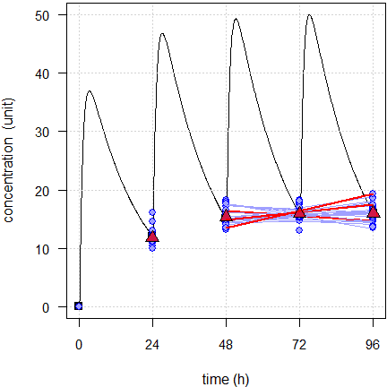
Fig. 1 First 24 of the simulated subjects, \(\small{CV=10\%}\).
Blue lines estimated regressions, red lines with significant slope, red triangles geometric means, black line model of build-up, black squares its pre-dose concentrations.
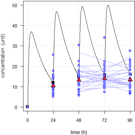
Fig. 2 First 24 of the simulated subjects, \(\small{CV=40\%}\).
Blue lines estimated regressions, red triangles geometric means, black line model of build-up, black squares its pre-dose concentrations.
Here with low variability three simulated subjects show a significant slope (FPR 12.5%) and with high variability none. When assessing the Durbin–Watson test, we find a significant autocorrelation in six simulated subjects with low variability and in five with high variability. Hence, it confirms that applying a regression is not justified.
Of course, in reality the level of the true steady state is unknown. The geometric means show that the pre-dose concentrations are stable, though with low variability they seem to rise a bit.
A shorter build-up (fewer doses) might be risky. Here planned with five half lives as recommended in the guidelines (only four doses, last dosing time rounded up from 60 to 72 hours).
10,000 simulations, linear model: C ~ a + b * t
 delta = 0.2 (acceptance limits {-delta, +delta})
 slope of model = +0.07828
 last model’s pre-dose concentration = 15.78
 CV = 10.0%, median of slopes = +0.07712
   97.3% positive slopes
    2.7% negative slopes
   significant slopes:   9.46% (95% CI does not contain zero)
   failed slopes     :  85.79% (95% CI not within acceptance limits)
   autocorrelation   :   6.2%
 CV = 40.0%, median of slopes = +0.06995
   68.9% positive slopes
   31.1% negative slopes
   significant slopes:   4.98% (95% CI does not contain zero)
   failed slopes     :  96.26% (95% CI not within acceptance limits)
   autocorrelation   :   4.4%
The positive slopes are detected. With low variability 9.46% is clearly above the level of the test. With high variability we are close to the level of the test.
As before, we assess a small subset.
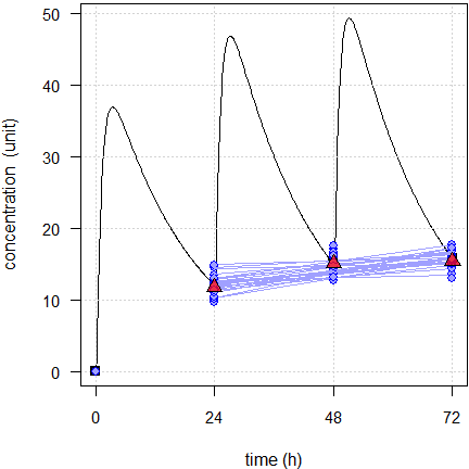
Fig. 3 First 24 of the simulated subjects, \(\small{CV=10\%}\).
Blue lines estimated regressions, red triangles geometric means, black line model of build-up, black squares its pre-dose concentrations.

Fig. 4 First 24 of the simulated subjects, \(\small{CV=40\%}\).
Blue lines estimated regressions, red line with significant slope, red triangles geometric means, black line model of build-up, black squares its pre-dose concentrations.
With low variability none of the simulated subjects show a significant slope and with high variability one. However, what might a regulatory assessor conclude? With low variability all slopes are positive and with high variability still 19.
An example from my files: A drug with polymorphic metabolism (\(\small{CV_\textrm{inter}\gg CV_\textrm{intra}}\)). Given the wide range of half lives reported in the literature and observed in our single dose studies, we dosed OAD for 14 days, translating into an average of 15.5 half lives (minimum 5.2, maximum 46). \[\small{\textrm{PK metric (ng/mL): }\bar{x}_\textrm{geom}\;(CV)}\]\[\small{ \begin{array}{lccc} \textrm{Treatment} & C_\textrm{pd} & C_\textrm{min} & C_\tau\\\hline \textrm{Test} & 28.47\;(80\%) & 26.99\;(79\%) & 33.41\;(59\%)\\ \textrm{Reference} & 29.80\;(77\%) & 28.19\;(75\%) & 32.84\;(61\%)\\\hline \end{array}}\]\(\small{C_\textrm{pd}>C_\textrm{min}}\), since in 26 of the 56 profiles we observed a lag time. Recall the accumulation example above. It is common that \(\small{C_\tau>C_\textrm{pd}}\) because we can never attain true steady state.
Although not assessed in the study, all of these PK metrics would pass conventional bioequivalence. \[\small{\begin{array}{lccccc} \textrm{PK metric} & PE & 90\%\;CL_\textrm{lo} & 90\%\;CL_\textrm{hi} & CV_\textrm{intra} & CV_\textrm{inter}\\\hline \phantom{000}C_\textrm{pd} & \phantom{1}95.54\% & 81.29\% & 112.29\% & 39.5\% & 133.3\%\\ \phantom{000}C_\textrm{min} & \phantom{1}95.74\% & 81.82\% & 112.03\% & 38.3\% & 128.2\%\\ \phantom{000}C_\tau & 100.48\% & 90.27\% & 111.85\% & 25.7\% & \phantom{1}94.3\%\\\hline \end{array}}\] Here the results of the first period.
linear model: C ~ a + b * t
Δ = 0.5 (acceptance limits {–Δ, +Δ})
  42.9% positive slopes
  57.1% negative slopes
  significant slopes:  3.57% (95% CI does not contain zero)
  failed slopes     : 82.14% (95% CI not within acceptance limits)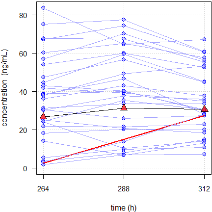
Fig. 5 Spaghetti plot of a CNS-drug in 28 subjects.
Red line regression with significant slope, red triangles geometric means.
The one subject with a significant slope (with a 95%
CI of 0.0039 – 1.038 it was a
close shave) had low variability. However, at the end of the profile day
the concentration was lower than at 312 hours. Hence, it is reasonable
to conclude that the subject was in steady state and the apparently
rising concentrations were due to pure chance. There was yet another
subject with a similar slope. Since its variability was higher, the
slope was not significant.
Note that ≈82% would fail even with an extremely liberal \(\small{\Delta=0.5}\).
According to the protocol we reported only individual data, descriptive statistics,11 individual and spaghetti plots. All European regulatory assessors were fine with that.
Interlude: Flip-flop Pharmacokinetics
\(\small{k_{10}}\): elimination rate constant
Even in a simple one-compartment model \(\small{k_{01}}\) and \(\small{k_{10}}\) are not identifiable. Where for IR formulations it is reasonable to assume \(\small{k_{10}\ll k_{01}}\), i.e., that absorption is much faster than elimination, for prolonged release formulations this must not be – and very likely is not – the case. If you are a dinosaur of biopharmaceutics like me, perhaps you remember the slogan of the 1980s »the flatter is better«. A main target of product development is to decrease \(\small{k_{01}}\) (increase the absorption half life). Never plan the study based on the apparent elimination half life of an IR formulation.
Here an example of flip-flop PK with \(\small{k_{01}=k_{10}=\textsf{8 h}}\), designed with the naïve dosing of seven elimination half lives (56 rounded up to 72 hours).
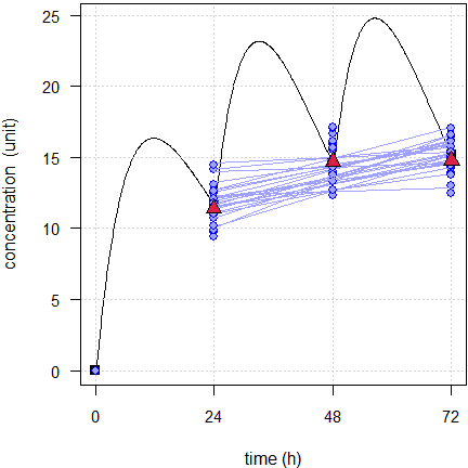
Fig. 6 24 simulated subjects, \(\small{CV=10\%}\).
Blue lines estimated regressions, red triangles geometric means, black line model of build-up, black squares its pre-dose concentrations.
That’s a recipe for disaster – all slopes are positive. Although none
is significantly different from zero, it would need a blind assessor to
accept a claim that steady state was achieved. And they would be
absolutely right. We would need dosing for ten half lives to
end up with something similar to Fig. 1.
As usual: Know the drug and know your formulation!
Power model
Given the behavior of the build-up, which is concave, one might be tempted set up a power model \[Y=a\cdot X^{\,b}+\epsilon\small{\textsf{.}}\tag{3}\] Like in dose-proportionality21 for convenience its linearized form \[\log_{e}Y=\log_{e}a+b\cdot\log_{e}X+\epsilon \tag{4}\] can be fitted. The tests are the same like in the linear model \(\small{(2)}\).
nsims  <- 1e4L # number of simulations
D      <- 200L # dose
f      <- 2/3  # fraction absorbed (BA)
V      <- 3    # volume of distribution
t12.a  <- 0.75 # absorption half life
t12.e  <- 12   # elimination half life
tlag   <- 0.25 # lag time
tau    <- 24L  # dosing interval
fact   <- 5L   # half life factor
CV.lo  <- 0.10 # drug with low variability
CV.hi  <- 0.40 # drug with high variability
delta  <- 0.2  # for acceptance limits = {1 - delta, 1 + delta}
dw     <- TRUE # Assess autocorrelation
method <- "power"
sim.ss(nsims, f, D, V, t12.a, t12.e, tlag, tau, fact,
       CV.lo, CV.hi, dw = dw, method = method)
# 10,000 simulations, power model: C ~ a * t^b
# delta = 0.2 (acceptance limits {-delta, +delta})
# exponent of model = +0.25554
# last model’s pre-dose concentration = 15.78
# CV = 10.0%, median of exponents = +0.25334
# 97.8% positive exponents
# 2.2% negative exponents
# significant exponents: 11.55% (95% CI does not contain zero)
# failed exponents : 98.88% (95% CI not within acceptance limits)
# autocorrelation : 12.2%
# CV = 40.0%, median of exponents = +0.25455
# 69.9% positive exponents
# 30.1% negative exponents
# significant exponents: 5.23% (95% CI does not contain zero)
# failed exponents : 99.59% (95% CI not within acceptance limits)
# autocorrelation : 10.8%Do we gain something? Not really.
As above the subset of 24 subjects.

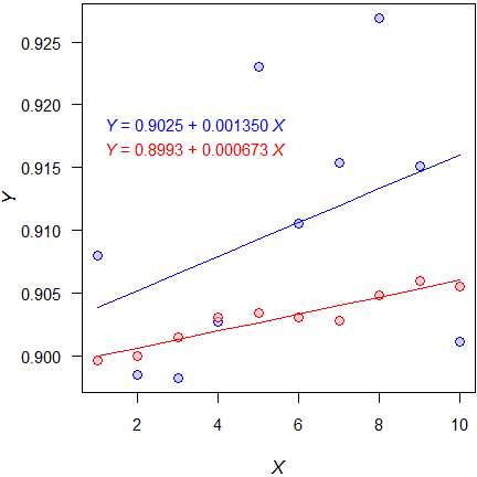
Fig. 7 First 24 of the simulated subjects, \(\small{CV=10\%}\).
Blue lines estimated regressions, red triangles geometric means, black line model of build-up, black squares its pre-dose concentrations.
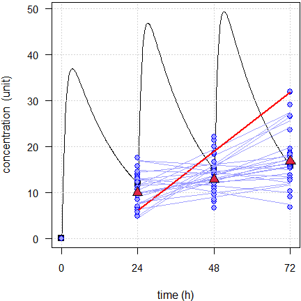
Fig. 8 First 24 of the simulated subjects, \(\small{CV=40\%}\).
Blue lines estimated regressions, red line with significant slope, red triangles geometric means, black line model of build-up, black squares its pre-dose concentrations.
We would arrive at the same conclusion than with the linear model. If we run both models we see that in some cases the power model fits better (based on an ANOVA or the AIC). However, we see also that some fits are convex and that is from a theoretical perspective simply wrong. That’s a dead end.
Alternative?
So why are we not fitting the function \[C=C_\textrm{ss}\big{(}1-\exp(-\lambda \times t)\big{)} \tag{5}\] underlying the build-up directly? There are two problems, a technical and a theoretical one.
We cannot linearize \(\small{(5)}\) like we did with the
power model \(\small{(3)}\). Hence, we require
nonlinear modeling as provided in R’s function
nls(), which requires suitable start values. In many cases
\(\small{\max (C) \Rightarrow
C_\textrm{ss}}\) and \(\small{\log_{e}2\,/\,t_{1/2}\Rightarrow\lambda}\)
work. Alternatively we can set up the model in Phoenix WinNonlin.
However, in most cases calculating a
CI fails.
Even if we obtain a CI,
which parameter should we test and against what?
The true steady state is unknown and therefore, testing \(\small{\widehat{C_\textrm{ss}}}\) is not an
option. We face a similar problem with testing \(\small{\widehat{\lambda}}\). We have only
the half life used in study planning and no clue what the subjects’ true
predominant rate constants are.
Summary
“NCA and statistics associated with either Ctrough or dosing interval PK parameters have limited value for SS characterization.
Ctrough is not very sensitive to characterize steady state (SS), especially for compounds that attained steady state slowly.
Testing for a significant difference is as flawed as a similar
approach in the early 1980s in bioequivalence was.
A large difference with high variability passes and a small difference
with low variability fails:
–0.00113, +0.00383, +0.000483, +0.000864
Assessing the CI would only make sense if there would be a priori defined acceptance limits. Such limits were never defined. Even an extremely liberal \(\small{\Delta\,0.5}\) does not work because the pre-dose concentrations are too variable. In the example above 83.73% would fail with low variability and 97.46% with high variability.
As we have seen in the simulations, we can get caught in the trap of false positives. Consequently we would exclude subjects and loose power. On the other hand, esp. with high variability, we would keep subjects which are not in steady state.
Too few doses (say, based on five times the half life) might not be a
good idea. With low variability we will be punished by slopes
significantly different from zero and even with high variability the
plots will be telling.
This exercise is not just about making assessors happy. Based on the
superposition principle23 of
PK we must compare
bioavailabilities only after a single dose or in
(pseudo-)steady state – not in the saturation phase between. Such a
comparison would be meaningless.
Recall the legal definition of bioequivalence in the U.S.A.:
“Two drug products will be considered bioequivalent drug products if they are pharmaceutical equivalents or pharmaceutical alternatives whose rate and extent of absorption do not show a significant difference when administered at the same molar dose of the active moiety under similar experimental conditions, either single dose or multiple dose.
Does that require testing for a statistically significant difference? Of course, not. It is meant in the simple language lawyers can comprehend.
“significant:
Large enough to be noticed or have an effect, having or likely to have influence or effect.
Similarly here when it comes to ‘demonstration’.
“demonstration:
An event that proves a fact.
‘Demonstration of steady state’ should not be understood in the statistical sense. Instead, individual pre-dose concentrations should be reported together with spaghetti plots and plots of geometric means.
In the discussion it became clear that common sense should prevail. Kudos!Recall that this was consistent with the EMA’s previous point of view11 that
»a […] statistical method is not considered necessary […]. Descriptive data is sufficient.«
If you insist in using a statistical approach, estimate the correlation between pre-dose concentrations by a mixed-effects model with subject as a random effect.26 Good luck – there is no guarantee that it will converge!
“[…] all models are approximations.
Essentially, all models are wrong, but some are useful.
I strongly hold that for ‘demonstrating achievement of steady state’ none of the proposed statistical models is useful at all…
Postscript
The requirement of multiple dose studies is highly controversial. At the time being the EMA – apart from Australia – is the only jurisdiction requiring them. They were never necessary for the FDA, and Health Canada required them only for drugs with accumulation (\(\small{AUC_{0-\tau}>80\%\,AUC_{0-\infty}}\)) until 2012.

Extensive simulations28 showed that comparing the concentration at the end of the intended dosing interval (\(\small{C_\tau}\)) – additionally to \(\small{AUC_{0-\text{t}}}\) and \(\small{C_\textrm{max}}\) – could reliably predict the outcome after multiple doses.
The approach comes with a price: Since \(\small{C_\tau}\) is a one-point metric and hence, likely the one with the largest variability of the entire profile, the sample size has to be increased in order to preserve power. Nevertheless, the perspective to waive the multiple dose study is appealing.
It must be mentioned that the publication won the AAPS’ »Clinical Pharmacology and Translational Research«Outstanding Manuscript Award in Modeling and Simulation
in 2012…
The proposal was challenged by a retrospective analysis29 of studies submitted to the Spanish agency AEMPS. The authors concluded that \(\small{C_\tau}\) after a single dose is a poor predictor of \(\small{C_\textrm{min,ss}}\) after multiple doses.
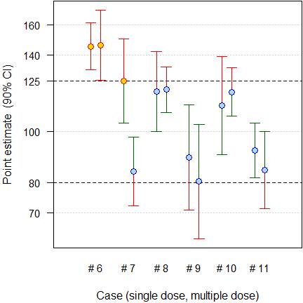
Fig. 10 Six cases which failed both after a single and after multiple doses.
“[…] in […] six cases […] the multiple dose study was the only [sic] design able to detect the differences and, therefore, it was essential when comparing the in vivo performance of prolonged release products.
Regarding the predictive value of \(\small{C_\tau}\), one case […] shows that it is predictive of the bioequivalence failure of \(\small{C_\textrm{min,ss}}\), but in the other five cases, the results are not predictive or as sensitive as \(\small{C_\textrm{max,ss}}\) or \(\small{C_\textrm{min,ss}}\).
Regrettably, only failed studies were reported and therefore, it is not possible to assess the FPR. I’m not a friend of post hoc power, but evidently none [sic] of the studies was sufficiently powered (median 11.84%, quartiles 3.25 – 13.35%) to demonstrate BE for this metric. That is not surprising, since assessing \(\small{C_\tau}\) was not a regulatory requirement at submission. In short, the results do not refute but rather support the simulation study: All cases which failed after a single dose failed after multiple doses as well. Not only the data base is obscure but – more importantly – the authors’ conclusions contradict their findings. That’s bad in an age when many people don’t read publications beyond its abstract. Alas, the paper is cited as ‘evidence’ to support the need of multiple dose studies.
The paper was defended30 and IMHO, understandably, challenged.31 32 33
“Science should always be the basis of regulatory requirements.
Given the limited data on new PK metrics, it was proposed at the »EUFEPS Open Discussion Forum«25 that regulations should not be made up out of thin air but based on science.
- BE should be assessed only by conventional PK metrics according to the (then) current guideline.
- Applicants should analyze studies with the suggested new PK metrics in an exploratory manner and submit results to agencies.
- After a limited time frame (e.g., two years) the data could be assessed for their sensitivity and included in the new guideline if deemed necessary.35
We all know how it ended. Although in April 201436 it was promised that »the overview of comments will be published within the next two weeks«, we had to wait for 5½ years.37 38 As usual, most suggestions were ignored.
The Brazilian competent authority ANVISA required multiple dose studies as well. The message was heard and hence, the agency retrospectively assessed 117 studies submitted since 2008 for early and late partial \(\small{AUC}\) (\(\small{\textrm{p}AUC_{0-\tau/2}}\), \(\small{\textrm{p}AUC_{\tau/2-\tau}}\)).39 79.2% of studies which passed conventional PK metrics, passed the partial \(\small{AUC\textrm{s}}\) as well. In order to pass, in general the sample size has not to be increased. Therefore, the requirement was lifted and only \(\small{C_\text{max}}\), \(\small{AUC_{0-\text{t}}}\), \(\small{\textrm{p}AUC_{0-\tau/2}}\), \(\small{\textrm{p}AUC_{\tau/2-\tau}}\) after a single dose are required. 18 40
Let us hope that – in the spirit of global harmonization – sooner or later the EMA (and its ‘disciples’ in Australia) will follow all other agencies.
“In advanced engineering, you expected failure; you learned as much from failures as from successes – indeed if you never suffered a failure you probably weren’t pushing the envelope ambitiously enough.
Licenses
 Helmut Schütz 2025
R and pandoc GPL 3.0,
klippy MIT.
1st version January 16, 2022. Rendered March 13, 2025 14:07
CET by rmarkdown via pandoc in 0.09 seconds.
Footnotes and References
Light RJ, Singer JD, Willett JB. By Design. Planning Research on Higher Education. Cambridge: Harvard University Press: 1990. ISBN 9780674089310. p. V.↩︎
Bonate PL. Pharmacokinetic-Pharmacodynamic Modeling and Simulation. New York: Springer; 2nd ed. 2011. p. 359.↩︎
Gabrielsson J, Weiner D. Pharmacokinetic and Pharmacodynamic Data Analysis: Concepts and Applications. Stockholm: Apotekarsocieteten; 5th ed. 2016. p. 335–6, p. 704.↩︎
Tóthfalusi L, Endrényi L. Approvable generic carbamazepine formulations may not be bioequivalent in target patient populations. Int J Clin Pharm Ther. 2013; 51(6). 525–8. doi:10.5414/CP201845.↩︎
Hauck WW, Tozer TN, Anderson S, Bois F. Considerations in the Attainment of Steady State: Aggregate vs. Individual Assessment. Pharm Res. 1998; 15(11): 1796–8. doi:10.1023/A:1011933401522.↩︎
EC. Investigation of bioavailability and bioequivalence. 3CC15a. Brussels. December 1991.
 BEBAC
Archive.↩︎
BEBAC
Archive.↩︎EMEA, CPMP. Note for guidance on modified release oral and transdermal dosage forms. Pharmacokinetic and clinical evaluation. London. 28 July 1999. Online.↩︎
EMEA, CPMP. Note for guidance on the investigation of bioavailability and bioequivalence. London. 26 July 2001. Online.↩︎
WHO Expert Committee on Specifications for Pharmaceutical Preparations, Fifty-first Report (WHO TRS No. 1003), Annex 6. Multisource (generic) pharmaceutical products: guidelines on registration requirements to establish interchangeability. Geneva. 2017. Online.↩︎
Health Canada, Health Products and Food Branch. Guidance for Industry. Conduct and Analysis of Bioavailability and Bioequivalence Studies – Part B: Oral Modified Release Formulations. Ottawa. 1996.
 Internet
Archive.↩︎
Internet
Archive.↩︎EMEA. Overview of Comments received on Draft Guideline on the Investigation of Bioequivalence. London. 20 January 2010. Online.↩︎
Health Canada. Guidance Document. Comparative Bioavailability Standards: Formulations Used for Systemic Effects. Adopted 2012/02/08, Revised 2023/01/30. Online.↩︎
FDA, CDER. Draft Guidance for Industry. Bioequivalence Studies With Pharmacokinetic Endpoints for Drugs Submitted Under an ANDA. Silver Spring. August 2021. Download.↩︎
Fang L. PK and Statistical Considerations for Steady State BE Studies – FDA Perspective. Presentation at SAAMnow Spring 2019 Workshop. Rockville. April 4–5, 2019. Online.↩︎
EMA, CHMP. Guideline on the pharmacokinetic and clinical evaluation of modified release dosage forms. London. 20 November 2014. Online.↩︎
TGA. International scientific guidelines adopted in Australia. Guideline on the pharmacokinetic and clinical evaluation of modified release dosage forms with TGA annotations. Canberra. 22 August 2024. Online.↩︎
ICH. Bioequivalence for Immediate Release Solid Oral Dosage Forms. M13A. Geneva. 23 July 2024. Online.↩︎
ANVISA. Resolução - RDC Nº 742. Dispõe sobre os critérios para a condução de estudos de biodisponibilidade relativa / bioequivalência (BD/BE) e estudos farmacocinéticos. Brasilia. August 10, 2022. Effective July 3, 2023. Online. [Portuguese]↩︎
Weimann HJ. Drug concentrations and directly derived parameters. In: Cawello W, editor. Parameters for Compartment-Free Pharmacokinetics. Aachen: Shaker-Verlag; 2003. p. 32.↩︎
I have to admit that I used to recommend it myself.↩︎
Wolfsegger MJ, Bauer A, Labes D, Schütz H, Vonk R, Lang B, Lehr S, Jaki TF, Engl W, Hale MD. Assessing goodness-of-fit for evaluation of dose-proportionality. Pharm Stat. 2021; 20(2): 272–81. doi:10.1002/pst.2074.↩︎
Nicolas X, Sultan E, Ollier C, Rauch C, Fabre D. Estimation by different techniques of steady-state achievement and accumulation for a compound with bi-phasic disposition and long terminal half-life. PAGE meeting. Montpellier. July 7–13, 2013. Online.↩︎
Dost FH. Der Blutspiegel. Konzentrationsabläufe in der Kreislaufflüssigkeit. Leipzig: VEB Thieme; 1953. p. 244. [German]↩︎
CFR. Title 21. Volume 5. Chapter I. §320.23 (b)(1) Basis for measuring in vivo bioavailability or demonstrating bioequivalence. Jan. 22, 2024. Online.↩︎
EUFEPS. Open Discussion Forum on the Revised European Guideline on Pharmacokinetic and Clinical Evaluation of Modified Release Dosage Forms. Bonn. 17–18 June, 2013.↩︎
Maganti L, Panebianco DL, Maes AL. Evaluation of Methods for Estimating Time to Steady State with Examples from Phase 1 Studies. AAPS J. 2008; 10(1): 141–7. doi:10.1208%2Fs12248-008-9014-y.
 Free
Full Text.↩︎
Free
Full Text.↩︎Box GEP, Draper NR. Empirical Model-Building and Response Surfaces. New York: Wiley; 1987. p. 424.↩︎
Paixão P, Gouveia LF, Morais JAG. An alternative single dose parameter to avoid the need for steady-state studies on oral extended-release drug products. Eur J Pharmaceut Biopharmaceut. 2012; 80(2): 410–7. doi:10.1016/j.ejpb.2011.11.001.↩︎
García-Arieta A, Morales-Alcelay S, Herranz M, de la Torre-Alvarado JM, Blázquez-Pérez A, Suárez-Gea ML, Alvarez C. Investigation on the need of multiple dose bioequivalence studies for prolonged-release generic products. Int J Pharm. 2012; 423(2): 321–5. doi:10.1016/j.ijpharm.2011.11.022.↩︎
García‐Arieta A. Justification of the current regulatory approach by EMA prohibiting the extrapolation of single dose BE to steady state in many cases. Presentation at: 3rd GBHI Workshop. Amsterdam. April 12, 2018.↩︎
Schütz H. Primary and secondary PK metrics for evaluation of steady state studies, \(\small{C_\text{min}}\) vs. \(\small{C_\tau}\), relevance of \(\small{C_\text{min}}\)/\(\small{C_\tau}\) or fluctuation for bioequivalence assessment. Presentation at: 3rd GBHI Workshop. Amsterdam; 12 April 2018. Online.↩︎
Silva N. Suggestions for Further Harmonization of Remaining Open Issues. GBHI, 4th International Workshop. Bethesda. December 12, 2019.↩︎
Cook J. Scientific Arguments in Favor and Against the Requirement to Perform Multiple Dose Studies for Long Acting Injectables and Implants. GBHI, 4th International Workshop. Bethesda. December 12, 2019.↩︎
Röhmel J. Recent Methodological Advances Contributing to Clinical Trials and Regulatory Statistics. 30th Annual Conference of the International Society for Clinical Biostatistics. Prague. August 25, 2009.↩︎
That’s similar to what the FDA did when concerns about the ‘Subject-by-Formulation’ interaction emerged. Temporarily studies had to be performed in a replicated design. After assessing the results, the FDA concluded that the S × F interaction is not relevant and the temporary requirement was lifted.↩︎
EMA/EGA. Joint workshop on the impact of the revised EMA Guideline on the Pharmacokinetic and Clinical Evaluation of Modified Release Dosage Forms. London. 30 April 2014.↩︎
EMA, PKWP. Overview of comments received on ‘Guideline on the pharmacokinetic and clinical evaluation of modified release dosage forms’. London. 17 October 2019. Online.↩︎
Regrettably it does not contain a column ‘Outcome’, which served well in other documents in understanding the EMA’s point of view.↩︎
Costa Soares KE, Chiann C, Storpitis S. Assessment of the impact of partial area under the curve in a bioavailability / bioequivalence study on generic prolonged-release formulations. Eur J Pharm Sci. 2022; 171: 106127. doi:10.1016/j.ejps.2022.106127.↩︎
Costa Soares KE (ANVISA/CETER). Presentation at: Multiple dose studies for generic and similar drugs of modified release. São Paulo. April 29, 2021. URL.↩︎
Baxter S. Transcendent. London: Gollanz; 2005. Chapter 36.↩︎