
Post hoc Power
Helmut Schütz

August 12, 2024
Consider allowing JavaScript. Otherwise, you have to be proficient in
reading  since formulas
will not be rendered. Furthermore, the table of contents in the left
column for navigation will not be available and code-folding not
supported. Sorry for the inconvenience.
since formulas
will not be rendered. Furthermore, the table of contents in the left
column for navigation will not be available and code-folding not
supported. Sorry for the inconvenience.
Examples in this article were generated with
 4.4.1 by the packages
 PowerTOST1 and
randomizeBE.2 See also the online manual3 for details.
The right-hand badges give the respective section’s ‘level’.
- Basics about power and sample size methodology – requiring no or only limited statistical expertise.
- These sections are the most important ones. They are – hopefully – also easy to understand for newcomers. A basic knowledge of R does not hurt.
- A somewhat higher knowledge of statistics and/or R is required. May be skipped or reserved for a later reading.
- An advanced knowledge of statistics and/or R is required. Not recommended for beginners in particular.
- Click to show / hide R code.
- Click on the icon
 in the top left corner to copy R code to the
clipboard.
in the top left corner to copy R code to the
clipboard.
Introduction
What is the purpose of calculating post hoc Power?
I will try to clarify why such a justification is meaningless and – a bit provocative – asking for one demonstrates a lack of understanding the underlying statistical concepts (see another article for details about inferential statistics and hypotheses in equivalence).
As an aside, in bioinformatics – where thousands of test are performed simultaneously – post hoc power is indeed a suitable tool to select promising hypotheses.4
In the case of a single test (like in bioequivalence) it has been
extensively criticized. 5 6 7
It may be of interest for the sponsor if another study is
planned.
“There is simple intuition behind results like these: If my car made it to the top of the hill, then it is powerful enough to climb that hill; if it didn’t, then it obviously isn’t powerful enough. Retrospective power is an obvious answer to a rather uninteresting question. A more meaningful question is to ask whether the car is powerful enough to climb a particular hill never climbed before; or whether a different car can climb that new hill. Such questions are prospective, not retrospective.
Preliminaries
A basic knowledge of R is
required. To run the scripts at least version 1.4.3 (2016-11-01) of
PowerTOST is suggested. Any version of R would likely do, though the current release of
PowerTOST was only tested with R
version 4.3.3 (2024-02-29) and later. At least version 0.3.1
(2012-12-27) of randomizeBE is required. All scripts were
run on a Xeon E3-1245v3 @ 3.40GHz (1/4 cores) 16GB RAM with R 4.4.1 on Windows 7 build 7601, Service Pack 1,
ucrt 10.0.10240.16390.
library(PowerTOST)   # attach required ones
library(randomizeBE) # to run the examples
top of section ↩︎ previous section ↩︎
Background
In order to get prospective (a priori) power \(\small{\pi}\) and hence, estimate a sample size, we need five values:
- The level of the test (in bioequivalence commonly \(\small{\alpha=0.05}\)),
- the BE-margins (commonly \(\small{80-125\%}\)),
- the desired (or target) power \(\small{\pi}\), where the producer’s risk of failure \(\small{\beta=1-\pi}\),
- the variance \(\small{s^2}\) (commonly expressed as a coefficient of variation \(\small{CV}\)), and
- the deviation \(\small{\Delta}\) of the test from the reference treatment.
1 & 2 are fixed by the
agency,
3 is set by the sponsor
(commonly to \(\small{80-90\%}\)),
and
4 & 5 are – uncertain! – assumptions.
The European Note for Guidance9 was specific in this respect:
“The number of subjects required is determined byUnfortunately the current guideline10 reduced this section to the elastic clause
- the error variance associated with the primary characteristic to be studied as estimated from a pilot experiment, from previous studies or from published data,
- the significance level desired,
- the expected deviation from the reference product compatible with bioequivalence (delta) and
- the required power.
May I ask what’s »appropriate«?
However, all of that deals with the design of the study. From a regulatory perspective the
outcome of a comparative
bioavailability study is dichotomous:
Either bioequivalence was demonstrated (the
\(\small{100(1-2\,\alpha)}\) confidence
interval lies entirely within the pre-specified acceptance range) or not.
- The patient’s risk is always strictly controlled (\(\small{\leq\alpha}\)).
- The actual producer’s risk \(\small{\widehat{\beta}}\) or post hoc (a.k.a. a posteriori, retrospective, estimated) power \(\small{\widehat{\pi}=1-\widehat{\beta}}\) do not play any role in this decision. An agency should not even ask for it because \(\small{\widehat{\beta}}\) is independent from \(\small{\alpha}\).
Since it is extremely unlikely that all assumptions made in designing the study will be exactly realized, it is of limited value to assess post hoc power – unless the study failed and one wants to design another one. More about that later.
top of section ↩︎ previous section ↩︎
Methods
Power Approach
The Power Approach11 (also known as the ‘80/20-rule’) consists
of testing the hypothesis of no difference (or a ratio of 1) at the
\(\small{\alpha}\) level of
significance (commonly 0.05). \[H_0:\;\frac{\mu_\text{T}}{\mu_\text{R}}=1\;vs\;H_1:\;\frac{\mu_\text{T}}{\mu_\text{R}}\neq
1,\tag{1}\] where \(\small{H_0}\) is the null
hypothesis of inequivalence and \(\small{H_1}\) the alternative
hypothesis of equivalence. \(\small{\mu_\text{T}}\) and \(\small{\mu_\text{R}}\) are the geometric
least squares means of \(\small{\text{T}}\) and \(\small{\text{R}}\), respectively. In order
to pass the test, the estimated (post hoc, a
posteriori, retrospective) power has to be at least 80%. The power
depends on the true value of \(\small{\sigma}\), which is unknown. There
exists a value of \(\small{\sigma_{\,0.80}}\) such that if
\(\small{\sigma\leq\sigma_{\,0.80}}\),
the power of the test of no difference \(\small{H_0}\) is greater or equal to 0.80.
Since \(\small{\sigma}\) is unknown, it
has to be approximated by \(\small{s}\). The Power Approach in a simple
2×2×2 crossover design then consists of rejecting \(\small{H_0}\) and concluding that \({\mu_\text{T}}\) and \({\mu_\text{R}}\) are equivalent if \[-t_{1-\alpha/2,\nu}\leq\frac{\bar{X}_\text{T}-\bar{X}_\text{R}}{s\sqrt{\tfrac{1}{2}\left(\tfrac{1}{n_1}+\tfrac{1}{n_2}\right)}}\leq
t_{1-\alpha/2,\nu}\:\text{and}\:s\leq\sigma_{0.80},\tag{2}\]
where \(\small{n_1,\,n_2}\) are the
number of subjects in sequences 1 and 2, the degrees of freedom \(\small{\nu=n_1+n_2-2}\), and \(\small{\bar{X}_\text{T}\,,\bar{X}_\text{R}}\)
are the \(\small{\log_{e}}\)-transformed means of
\(\small{\text{T}}\) and \(\small{\text{R}}\), respectively.
Note that this procedure is based on estimated power \(\small{\widehat{\pi}}\), since the
true power is a function of the unknown \(\small{\sigma}\). It was the only approach
based on post hoc power, was never implemented in any
jurisdiction except the
FDA, and is of
historical interest only.12
top of section ↩︎ previous section ↩︎
TOST Procedure
The Two One-Sided Tests Procedure11 consists of decomposing the interval hypotheses \(\small{H_0}\) and \(\small{H_1}\) into two sets of one-sided hypotheses with lower and upper limits \(\small{\left\{\theta_1,\,\theta_2\right\}}\) of the acceptance range based on a ‘clinically not relevant difference’ \(\small{\Delta}\) (commonly 20%). \[\begin{matrix}\tag{3} \theta_1=1-\Delta,\theta_2=\left(1-\Delta\right)^{-1}\\ H_{01}:\;\frac{\mu_\text{T}}{\mu_\text{R}}\leq\theta_1\;vs\;H_{11}:\;\frac{\mu_\text{T}}{\mu_\text{R}}>\theta_1\\ H_{02}:\;\frac{\mu_\text{T}}{\mu_\text{R}}\geq\theta_2\;vs\;H_{12}:\;\frac{\mu_\text{T}}{\mu_\text{R}}<\theta_2 \end{matrix}\] The TOST Procedure consists of of rejecting the interval hypothesis \(\small{H_0}\), and thus concluding equivalence of \(\small{\mu_\text{T}}\) and \(\small{\mu_\text{R}}\), if and only if both \(\small{H_{01}}\) and \(\small{H_{02}}\) are rejected at the significance level \(\small{\alpha}\).
top of section ↩︎ previous section ↩︎
CI Inclusion Approach
The two-sided \(\small{1-2\,\alpha}\) confidence interval is assessed for inclusion in the acceptance range.13 \[H_0:\;\frac{\mu_\text{T}}{\mu_\text{R}}\ni\left\{\theta_1,\theta_2\right\}\;vs\;H_1:\;\theta_1<\frac{\mu_\text{T}}{\mu_\text{R}}<\theta_2\tag{4}\]
top of section ↩︎ previous section ↩︎
Comparison
<nitpick>»bioequivalence was assessed by the Two One-Sided Tests (TOST) Procedure«
only to find that the Confidence Interval inclusion approach was actually emplyed. Although these approaches are operationally identical11 (their outcomes [pass | fail] are the same), these are statistically different methods:
- The TOST Procedure gives two \(\small{p-}\)values, namely \(\small{p(\theta_0\geq\theta_1)}\) and \(\small{p(\theta_0\leq\theta_2)}\). Bioequivalence is concluded if both \(\small{p}\)-values are \(\small{\leq\alpha}\).
- In the Confidence Interval Inclusion Approach bioequivalence is concluded if the two-sided \(\small{1-2\,\alpha}\) CI lies entirely within the acceptance range \(\small{\left\{\theta_1,\theta_2\right\}}\).
In 37 years, I haven’t seen a single study assessed by the
TOST Procedure.
One should stop referring to the
TOST Procedure, when the study
was assessed by the CI
Inclusion Approach – as required in all global guidelines since
1992 [sic].
</nitpick>
It must be mentioned that neither the TOST Procedure nor the CI Inclusion Approach are uniformly most powerful tests.14 However, none of the alternatives were ever implemented in any jurisdiction.
top of section ↩︎ previous section ↩︎
Examples
Let’s explore the properties of prospective power. Assumed CV 0.25, T/R-ratio 0.95, targeted at 90% power in a 2×2×2 crossover design:
alpha  <- 0.05
CV     <- 0.25
theta0 <- 0.95
theta1 <- 0.80
theta2 <- 1/theta1
target <- 0.90
design <- "2x2x2"
n      <- sampleN.TOST(alpha = alpha, CV = CV,
                       theta0 = theta0,
                       theta1 = theta1, theta2 = theta2,
                       targetpower = target,
                       design = design,
                       print = FALSE)[["Sample size"]]
pe     <- sort(unique(c(seq(theta1, 1, length.out = 100),
                        1/seq(theta1, 1, length.out = 100))))
res1   <- data.frame(pe = pe, p.left = NA, p.right = NA,
                     power = NA)
for (i in 1:nrow(res1)) {
  res1[i, 2:3] <- pvalues.TOST(pe = pe[i],
                               theta1 = theta1,
                               theta2 = theta2,
                               CV = CV, n = n,
                               design = design)
  res1[i, 4]   <- power.TOST(alpha = alpha,
                             theta0 = pe[i],
                             theta1 = theta1,
                             theta2 = theta2,
                             CV = CV, n = n,
                             design = design)
}
clr    <- c("#FF0000A0", "#FF00FFA0", "#0000FFA0")
dev.new(width = 4.5, height = 4.5)
op     <- par(no.readonly = TRUE)
par(mar = c(4, 4, 0, 0))
plot(pe, res1$power, type = "n", ylim = c(0, 1), log = "x",
     axes = FALSE, xlab = "", ylab = "")
abline(v = c(theta0, 1/theta0),
       h = c(alpha, 0.5), lty = 2)
grid()
box()
axis(1, at = c(seq(theta1, 1.2, 0.1), theta2))
axis(1, at = c(theta1, theta0, 1/theta0, theta2),
     tick = FALSE, line = 2,
     labels = c(expression(theta[1]),
                expression(theta[0]),
                expression(1/theta[0]),
                expression(theta[2])))
axis(2, las = 1)
mtext(expression(italic(p)* " / power"), 2, line = 3)
lines(pe, res1$p.left, col = clr[1], lwd = 3)
lines(pe, res1$p.right, col = clr[2], lwd = 3)
lines(pe, res1$power, col = clr[3], lwd = 3)
legend("center", box.lty = 0, bg = "white", y.intersp = 1.2,
       legend = c(expression(italic(p)>=theta[1]),
                  expression(italic(p)<=theta[2]),
                  "power"), col = clr, lwd = 3, seg.len = 3)
par(op)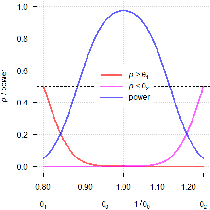
Fig. 1 Power curves for
n = 38.
With the assumed \(\small{\theta_0}\) of 0.9500 (and its reciprocal of 1.0526) we achieve the target power. If \(\small{\theta_0}\) will be closer to 1, we gain power. With \(\small{\theta_0}\) at the BE-margins \(\small{\left\{\theta_1,\theta_2\right\}}\) it will lead to a false decision (probability 0.05 of the Type I Error). Note that at the margins the respective p-value of the TOST procedure11 is 0.5 (like tossing a coin).
We can reverse this game and ask at which T/R-ratios power will be just 0.5 (with more deviating ones the chance to demonstrate BE is futile).
opt <- function(x) {
  power.TOST(theta0 = x, alpha = alpha,
             theta1 = theta1, theta2 = theta2,
             design = design,
             CV = CV, n = n) - 0.5
}
alpha  <- 0.05
CV     <- 0.25
theta0 <- 0.95
theta1 <- 0.80
theta2 <- 1/theta1
target <- 0.90
design <- "2x2x2"
n      <- sampleN.TOST(alpha = alpha, CV = CV,
                       theta0 = theta0,
                       theta1 = theta1, theta2 = theta2,
                       targetpower = target,
                       design = design,
                       print = FALSE)[["Sample size"]]
pe     <- sort(unique(c(seq(theta1, 1, length.out = 100),
                        1/seq(theta1, 1, length.out = 100))))
res1   <- data.frame(pe = pe, p.left = NA, p.right = NA,
                     power = NA)
for (i in 1:nrow(res1)) {
  res1[i, 2:3] <- pvalues.TOST(pe = pe[i],
                               theta1 = theta1,
                               theta2 = theta2,
                               CV = CV, n = n,
                               design = design)
  res1[i, 4]   <- power.TOST(alpha = alpha,
                             theta0 = pe[i],
                             theta1 = theta1,
                             theta2 = theta2,
                             CV = CV, n = n,
                             design = design)
}
pwr0.5 <- uniroot(opt, interval = c(theta1, theta0), tol = 1e-12)$root
clr    <- c("#FF0000A0", "#FF00FFA0", "#0000FFA0")
dev.new(width = 4.5, height = 4.5)
op     <- par(no.readonly = TRUE)
par(mar = c(4, 4, 0, 0))
plot(pe, res1$power, type = "n", ylim = c(0, 1), log = "x",
     axes = FALSE, xlab = "", ylab = "")
abline(v = c(pwr0.5, 1/pwr0.5),
       h = c(alpha, 0.5), lty = 2)
grid()
box()
axis(1, at = c(seq(theta1, 1.2, 0.1), theta2))
axis(1, at = c(theta1, pwr0.5, 1/pwr0.5, theta2),
     tick = FALSE, line = 2,
     labels = c(expression(theta[1]),
                expression(theta[0]),
                expression(1/theta[0]),
                expression(theta[2])))
axis(2, las = 1)
mtext(expression(italic(p)* " / power"), 2, line = 3)
lines(pe, res1$p.left, col = clr[1], lwd = 3)
lines(pe, res1$p.right, col = clr[2], lwd = 3)
lines(pe, res1$power, col = clr[3], lwd = 3)
legend("center", box.lty = 0, bg = "white", y.intersp = 1.2,
       legend = c(expression(italic(p)>=theta[1]),
                  expression(italic(p)<=theta[2]),
                  "power"), col = clr, lwd = 3, seg.len = 3)
par(op)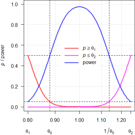
Fig. 2 Power curves for
n = 38.
We see that the extreme T/R-ratios are 0.8795 and 1.1371. At these T/R-ratios the respective p-value of the TOST is 0.05 and the null hypothesis of inequivalence has to be accepted. In other words, if we want to demonstrate BE for ‘worse’ T/R-ratios, we have to increase the sample size.
Misconceptions
As stated already above, post hoc power is not relevant in the assessment for BE. Consequently, it is not mentioned in any (‼) of the current global guidelines. The WHO argued against calculating it.15
“The a posteriori power of the study does not need to be calculated. The power of interest is that calculated before the study is conducted to ensure that the adequate sample size has been selected. […] The relevant power is the power to show equivalence within the pre-defined acceptance range.
top of section ↩︎ previous section ↩︎
‘Too low’ Power
To repeat: Either a study passed or it failed. If any of the assumptions in sample size planning (CV, T/R-ratio, anticipated dropout-rate) are not exactly realized in the study and turned out to be worse (e.g., higher CV, T/R-ratio deviating more from 1, less eligible subjects), post hoc power will be lower than targeted (\(\small{\widehat{\pi}<\pi}\)). Or simply:
“Being lucky is not a crime.
Since \(\small{\alpha}\) and \(\small{\widehat{\beta}}\) are independent, this is not of a regulatory concern (the patient’s risk is not affected).
Imagine: You visit a casino once in your life to play roulette and place a single bet of € 1,000 on the number 12 because that’s your birthday. The wheel spins and finally the ball drops into the 12-pocket of the wheel. Instead of paying out € 35,000 the croupier tells you with a smirk on his face:From the results of Example 2, Method B (the co-authors Walter Hauck and Donald Schuirmann are pioneers of statistics in bioequivalence):
“[…] we obtain a two-sided CI for the ratio (T/R) of geometric means of 88.45—116.38%, which meets the 80–125% acceptance criterion. We stop here and conclude BE, irrespective of the fact that we have not yet achieved the desired power of 80% (power = 66.3%).
Let’s consider an example. Assumed CV 0.30, T/R-ratio 0.95, targeted at 80% power in a 2×2×2 crossover design:
alpha     <- 0.05
CV        <- 0.30
theta0    <- 0.95
theta1    <- 0.80
theta2    <- 1/theta1
target    <- 0.80
design    <- "2x2x2"
plan      <- data.frame(CV = CV, theta0 = theta0,
                        n = NA, power = NA)
plan[3:4] <- sampleN.TOST(alpha = alpha, CV = CV,
                          theta0 = theta0,
                          theta1 = theta1, theta2 = theta2,
                          targetpower = target,
                          design = design,
                          print = FALSE)[7:8]
print(signif(plan, 4), row.names = FALSE)
# CV theta0 n power
# 0.3 0.95 40 0.8158So far, so good.
However, in the study the CV was higher (0.36), the Point Estimate worse (0.92), and we had two dropouts (38 eligible subjects).
alpha       <- 0.05
theta1      <- 0.80
theta2      <- 1/theta1
design      <- "2x2x2"
CV          <- 0.36 # higher than assumed
pe          <- 0.92 # more deviating than assumed
eligible    <- 38   # two dropouts
actual      <- data.frame(CV = CV, PE = pe, eligible = eligible,
                          lower.CL = NA, upper.CL = NA,
                          BE = "fail", power = NA, TIE = NA)
actual[4:5] <- sprintf("%.4f", CI.BE(alpha = alpha, CV = CV,
                                     pe = pe, n = eligible, design = design))
if (actual[4] >= theta1 & actual[5] <= theta2) actual$BE <- "pass"
actual[7]   <- sprintf("%.4f", power.TOST(alpha = alpha, CV = CV,
                                          theta0 = pe, n = eligible,
                                          design = design))
actual[8]   <- sprintf("%.6f", power.TOST(alpha = alpha, CV = CV,
                                          theta0 = theta1, n = eligible,
                                          design = design))
print(actual, row.names = FALSE)
# CV PE eligible lower.CL upper.CL BE power TIE
# 0.36 0.92 38 0.8036 1.0532 pass 0.5094 0.049933The study passed, though it was a close shave. What does the post hoc power of 0.5094 tell us what we don’t already know? Nothing. Is the patient’s risk compromised? Of course, not (0.049933 < 0.05).
‘Forced’ Bioequivalence
This is a term sometimes used by regulatory assessors.
Stop searching: You will not find it in any publication, textbook, or
guideline.
The idea behind: The sponsor had such a large budget, that the study was intentionally ‘overpowered’. What does that mean? Generally studies are powered to 80 – 90% (producer’s risk \(\small{\beta}\) 10 – 20%). That’s stated in numerous guidelines. If, say, the sponsor submitted a protocol aiming at 99% power to the IEC / IRB, it should have been rejected. Keep in mind that it is the responsibility of the IEC / IRB to be concerned about the safety of subjects in the study. If members voted in favor of performing the study, all is ‘good’. Regrettably, their statistical expertise is limited or it might have just slipped through their attention…
However, it might well be the opposite of what we discussed above. Say, the study was properly designed (prospective power \(\small{\pi\geq80\%}\)), but in the study the realized CV lower, the PE closer to 1, and the dropout-rate lower than the anticipated 10%.
up2even <- function(n) {
  return(as.integer(2 * (n %/% 2 + as.logical(n %% 2))))
}
nadj <- function(n, do.rate) {
  return(as.integer(up2even(n / (1 - do.rate))))
}
do.rate    <- 0.10 # 10%
plan       <- data.frame(state = "design", CV = 0.29, theta0 = 0.95,
                         target = 0.80, n = NA, power = NA)
plan[5:6]  <- sampleN.TOST(CV = plan$CV, theta0 = plan$theta0,
                           targetpower = plan$target, print = FALSE,
                           details = FALSE)[7:8]
plan[6]    <- sprintf("%.4f", plan[6])
plan$dosed <- nadj(plan$n, do.rate)
actual     <- data.frame(state = " study", CV = 0.24, PE = 0.99, n = 43,
                         lower.CL = NA, upper.CL = NA, BE = "fail",
                         power = NA)
actual[5:6] <- sprintf("%.4f", suppressMessages(
                                 CI.BE(CV = actual$CV,
                                       pe = actual$PE,
                                       n = actual$n)))
if (actual[4] >= 0.80 & actual[5] <= 1.25) actual$BE <- "pass"
actual[8] <- sprintf("%.4f", suppressMessages(
                               power.TOST(CV = actual$CV,
                                          theta0 = actual$PE,
                                          n = actual$n)))
names(actual)[4] <- "eligible"
print(plan, row.names = FALSE)
print(actual, row.names = FALSE)
# state CV theta0 target n power dosed
# design 0.29 0.95 0.8 38 0.8202 44
# state CV PE eligible lower.CL upper.CL BE power
# study 0.24 0.99 43 0.9085 1.0788 pass 0.9908Natually, post hoc power (\(\small{\widehat\pi}\)) was substantally
higher than targeted a priori (\(\small{\pi}\)). Again, it is not
of a regulatory concern (the patient’s risk is not affected).
Don’t you believe it? Calculate the probability of the Type I
Error (i.e., the probability that the null hypothesis of
bioinequivalence is true) by setting \(\small{\theta_0=\theta_1}\) or \(\small{\theta_0=\theta_2}\).
eligible <- 43
tie      <- data.frame(CV = actual$CV, eligible = eligible,
                       theta0 = c(0.80, 1.25), p = NA_real_)
tie$p[1] <- suppressMessages(
              power.TOST(CV = actual$CV, theta0 = 0.80,
                         n = eligible))
tie$p[2] <- suppressMessages(
              power.TOST(CV = actual$CV, theta0 = 1.25,
                         n = eligible))
names(tie)[4] <- "p (null = true)"
print(tie, digits = 13, row.names = FALSE)
# CV eligible theta0 p (null = true)
# 0.24 43 0.80 0.04999999999812
# 0.24 43 1.25 0.04999999999812In BE the pharmacokinetic metrics
\(\small{C_\textrm{max}}\) and \(\small{AUC_{0-\textrm{t}}}\) are mandatory
(in some jurisdictions like the
FDA additionally
\(\small{AUC_{0-\infty}}\)).
We don’t have to worry about multiplicity issues (an inflated Type I
Error leading to an increased patient’s risk), since if all
tests must pass at level \(\small{\alpha}\), we are protected by the
intersection-union principle.14 18
We design studies always for the worst case combination, i.e., driven by the PK metric requiring the largest sample size.
metrics <- c("Cmax", "AUCt", "AUCinf")
alpha   <- 0.05
CV      <- c(0.25, 0.19, 0.20)
theta0  <- c(0.95, 0.95, 0.95)
theta1  <- 0.80
theta2  <- 1 / theta1
target  <- 0.80
design  <- "2x2x2"
plan    <- data.frame(metric = metrics, CV = CV,
                      theta0 = theta0, n = NA, power = NA)
for (i in 1:nrow(plan)) {
  plan[i, 4:5] <- signif(
                    sampleN.TOST(alpha = alpha,
                                 CV = CV[i],
                                 theta0 = theta0[i],
                                 theta1 = theta1,
                                 theta2 = theta2,
                                 targetpower = target,
                                 design = design,
                                 print = FALSE)[7:8], 4)
}
txt     <- paste0("Sample size driven by ",
                  plan$metric[plan$n == max(plan$n)], ".\n")
print(plan, row.names = FALSE)
cat(txt)
# metric CV theta0 n power
# Cmax 0.25 0.95 28 0.8074
# AUCt 0.19 0.95 18 0.8294
# AUCinf 0.20 0.95 20 0.8347
# Sample size driven by Cmax.Say, we dosed more subjects to adjust for an anticipated dropout-rate of 10%. Let’s assume that all of our assumptions were exactly realized for \(\small{C_\textrm{max}}\) and were slightly ‘better’ for the \(\small{AUC \textrm{s}}\). There were two dropouts.
up2even <- function(n) {
  # round up to the next even number to get balanced sequences
  return(as.integer(2 * (n %/% 2 + as.logical(n %% 2))))
}
nadj <- function(n, do.rate) {
  return(as.integer(up2even(n / (1 - do.rate))))
}
metrics <- c("Cmax", "AUCt", "AUCinf")
alpha   <- 0.05
CV      <- c(0.25, 0.17, 0.18)
pe      <- c(0.95, 0.97, 0.96)
do.rate <- 0.1 # anticipated droput-rate 10%
n.adj   <- nadj(plan$n[plan$n == max(plan$n)], do.rate)
n.elig  <- n.adj - 2 # two dropouts
theta1  <- 0.80
theta2  <- 1 / theta1
actual  <- data.frame(metric = metrics,
                      CV = CV, PE = pe, n = n.elig,
                      lower.CL = NA, upper.CL = NA,
                      BE = "fail", power = NA, TIE = NA)
for (i in 1:nrow(actual)) {
  actual[i, 5:6] <- sprintf("%.4f", CI.BE(alpha = alpha,
                                          CV = CV[i],
                                          pe = pe[i],
                                          n = n.elig,
                                          design = design))
  if (actual[i, 5] >= theta1 & actual[i, 6] <= theta2)
    actual$BE[i] <- "pass"
  actual[i, 8] <- sprintf("%.4f", power.TOST(alpha = alpha,
                                             CV = CV[i],
                                             theta0 = pe[i],
                                             n = n.elig,
                                             design = design))
  actual[i, 9] <- sprintf("%.9f", power.TOST(alpha = alpha,
                                             CV = CV[i],
                                             theta0 = theta2,
                                             n = n.elig,
                                             design = design))
}
print(actual, row.names = FALSE)
# metric CV PE n lower.CL upper.CL BE power TIE
# Cmax 0.25 0.95 30 0.8526 1.0585 pass 0.8343 0.049999898
# AUCt 0.17 0.97 30 0.9007 1.0446 pass 0.9961 0.050000000
# AUCinf 0.18 0.96 30 0.8876 1.0383 pass 0.9865 0.050000000Such results are common in BE. As always, the patient’s risk is ≤ 0.05.
I have seen deficiency letters by regulatory assessors asking for aOutright bizarre.
Another case is common in jurisdictions accepting reference-scaling only for \(\small{C_\textrm{max}}\) (e.g. by Average Bioequivalence with Expanding Limits). Then regularly the sample size is driven by \(\small{AUC}\).
metrics <- c("Cmax", "AUCt", "AUCinf")
alpha   <- 0.05
CV      <- c(0.45, 0.34, 0.36)
theta0  <- rep(0.90, 3)
theta1  <- 0.80
theta2  <- 1 / theta1
target  <- 0.80
design  <- "2x2x4"
plan    <- data.frame(metric = metrics,
                      method = c("ABEL", "ABE", "ABE"),
                      CV = CV, theta0 = theta0,
                      L = 100*theta1, U = 100*theta2,
                      n = NA, power = NA)
for (i in 1:nrow(plan)) {
  if (plan$method[i] == "ABEL") {
    plan[i, 5:6] <- round(100*scABEL(CV = CV[i]), 2)
    plan[i, 7:8] <- signif(
                      sampleN.scABEL(alpha = alpha,
                                     CV = CV[i],
                                     theta0 = theta0[i],
                                     theta1 = theta1,
                                     theta2 = theta2,
                                     targetpower = target,
                                     design = design,
                                     details = FALSE,
                                     print = FALSE)[8:9], 4)
}else {
    plan[i, 7:8] <- signif(
                      sampleN.TOST(alpha = alpha,
                                   CV = CV[i],
                                   theta0 = theta0[i],
                                   theta1 = theta1,
                                   theta2 = theta2,
                                   targetpower = target,
                                   design = design,
                                   print = FALSE)[7:8], 4)
  }
}
txt <- paste0("Sample size driven by ",
              plan$metric[plan$n == max(plan$n)], ".\n")
print(plan, row.names = FALSE)
cat(txt)
# metric method CV theta0 L U n power
# Cmax ABEL 0.45 0.9 72.15 138.59 28 0.8112
# AUCt ABE 0.34 0.9 80.00 125.00 50 0.8055
# AUCinf ABE 0.36 0.9 80.00 125.00 56 0.8077
# Sample size driven by AUCinf.If the study is performed with 56 subjects (driven by \(\small{AUC_{0-\infty}}\)) and all assumed values are realized, post hoc power will be 0.9666 for \(\small{C_\textrm{max}}\).
Wrong Calculation
Post hoc power of the CI inclusion approach (or post hoc power of the TOST) has nothing to do with estimated power of testing for a statistically significant difference of 20% (the FDA’s dreadful 80/20-rule of 197211 12 outlined above). In the latter the realized (observed) PE is ignored [sic] and estimated power depends only on the CV and the residual degrees of freedom. Consequently, the estimated power will be practically always higher than the correct post hoc power.19
alpha    <- 0.05
CV       <- 0.25
theta0   <- 0.95
theta1   <- 0.80
theta2   <- 1/theta1
target   <- 0.80
design   <- "2x2x2"
n        <- sampleN.TOST(alpha = alpha, CV = CV,
                         theta0 = theta0,
                         theta1 = theta1, theta2 = theta2,
                         targetpower = target, design = design,
                         print = FALSE)[["Sample size"]]
pe       <- 0.89
res      <- data.frame(PE = pe, lower = NA, upper = NA,
                       p.left = NA, p.right = NA,
                       power.TOST = NA, power.20 = NA)
res[2:3] <- CI.BE(alpha = alpha, pe = pe,
                  CV = CV, n = n, design = design)
res[4:5] <- pvalues.TOST(pe = pe, CV = CV, n = n,
                         design = design)
res[6]   <- power.TOST(alpha = alpha, theta0 = pe,
                       theta1 = theta1, theta2 = theta2,
                       CV = CV, n = n, design = design)
res[7]   <- power.TOST(alpha = alpha, theta0 = 1,
                       theta1 = theta1, theta2 = theta2,
                       CV = CV, n = n, design = design)
names(res)[4:7] <- c("p (left)", "p (right)", "post hoc", "80/20-rule")
print(signif(res, 4), row.names = FALSE)
# PE lower upper p (left) p (right) post hoc 80/20-rule
# 0.89 0.7955 0.9957 0.05864 1.097e-05 0.4729 0.9023In this example the study failed (although properly planned for an
assumed T/R-ratio of 0.95, CV 0.25, targeted at 80%), because
the realized PE was only 89% and
hence, the lower 90% confidence limit just 79.55%. If you prefer the
TOST, the study failed because
\(\small{p(PE\geq\theta_1)}\) was with
0.05864 > 0.05 and the null hypothesis of inequivalence could not be
rejected. Like in any failed study, post hoc power was with
47.29% < 50%.
A ‘power’ of 90.23% is not even wrong.
If it really would have been that high, why on earth did the study fail?
Amazingly, such false results are all too often still seen in study
reports.
An example, where a study with the 90% CI-inclusion approach (as implemented in all global guidelines since the early 1990s!) or with the TOST would pass, but fail with the crappy 80/20-rule.
alpha    <- 0.05
CV.ass   <- 0.25 # assumed in designing the study
CV.real  <- 0.29 # realized (observed) in the study
theta0   <- 0.95
theta1   <- 0.80
theta2   <- 1/theta1
target   <- 0.80
design   <- "2x2x2"
n        <- sampleN.TOST(alpha = alpha, CV = CV.ass,
                         theta0 = theta0,
                         theta1 = theta1, theta2 = theta2,
                         targetpower = target, design = design,
                         print = FALSE)[["Sample size"]]
pe       <- 0.95 # same as assumed, we are lucky
res      <- data.frame(PE = pe, lower = NA, upper = NA,
                       p.left = NA, p.right = NA,
                       power.TOST = NA, power.20 = NA)
res[2:3] <- CI.BE(alpha = alpha, pe = pe,
                  CV = CV.real, n = n, design = design)
res[4:5] <- pvalues.TOST(pe = pe, CV = CV.real, n = n,
                         design = design)
res[6]   <- power.TOST(alpha = alpha, theta0 = pe,
                       theta1 = theta1, theta2 = theta2,
                       CV = CV.real, n = n, design = design)
res[7]   <- power.TOST(alpha = alpha, theta0 = 1,
                       theta1 = theta1, theta2 = theta2,
                       CV = CV.real, n = n, design = design)
names(res)[4:7] <- c("p (left)", "p (right)", "post hoc", "80/20-rule")
print(signif(res, 4), row.names = FALSE)
# PE lower upper p (left) p (right) post hoc 80/20-rule
# 0.95 0.8346 1.081 0.01612 0.0006349 0.6811 0.7758The study was planned as above, the
PE exactly as assumed, but the
realized CV turned out to be worse than assumed (29% instead of
25%). The 90% CI lies entirely
within 80.00–125.00% (alternatively, both \(\small{p}\)-values of the
TOST are < 0.05). Thus, the
null hypothesis of inequivalence is rejected and bioequivalence
concluded. The – irrelevant – post hoc power is 68.11%. It does
not matter that it is lower than the target of 80%, because the sample
size was planned based on assumptions.
In the ‘dark ages’ of bioequivalence (37 years ago…) the study would
have failed, because power to detect a 20% difference was with
77.58% less than 80%.
In Phoenix WinNonlin20 v6.4 (2014) Power_TOST21 was
introduced. During development22 it was cross-validated against the
function power.TOST(method = "nct")23 of the R package PowerTOST.1
Thankfully, the 80/20-rule20 was
abandoned by the
FDA in 1992,24 after
Schuirmann11 demonstrated that it is
flawed.25 Although it was never implemented in any
other jurisdiction, Power_80_20 is still available for
backwards compatibility in the current version 8.4.0 of Phoenix
WinNonlin.26 If you were guilty of using it in the
past, revise your procedures. Or even better: Stop
reporting post hoc power at all.
In PKanalix post hoc power is not calculated.27 Kudos!
Informative?
Post hoc power is an information sink.
Say, we test in a pilot study three candidate formulations \(\small{A,B,C}\) against reference \(\small{D}\). We would select the candidate with \(\small{\min\left\{\left|\log_{e}\theta_\textrm{A}\right|,\left|\log_{e}\theta_\textrm{B}\right|,\left|\log_{e}\theta_\textrm{C}\right|\right\}}\) for the pivotal study because it is the most promising one. If two T/R-ratios (or their reciprocals) are similar, we would select the candidate with the lower CV.
Let’s simulate a study in a 4×4 Williams’ design and evalute it according to the ‘Two at a Time’ approach (for details see the article about Higher-Order Crossover Designs). Cave: 257 LOC.
make.structure <- function(treatments = 3,
                           sequences = 6,
                           seqs, n, williams = TRUE,
                           setseed = TRUE) {
  # seq: vector of sequences (optional)
  # n  : number of subjects
  if (treatments < 3 | treatments > 5)
    stop("Only 3, 4, or 5 treatments implemented.")
  if (williams) {
    if (!sequences %in% c(4, 6, 10))
      stop("Only 4, 6, or 10 sequences in Williams\u2019 ",
           "designs implemented.")
    if (treatments == 3 & !sequences == 6)
      stop("6 sequences required for 3 treatments.")
    if (treatments == 4 & !sequences == 4)
      stop("4 sequences required for 4 treatments.")
    if (treatments == 5 & !sequences == 10)
      stop("10 sequences required for 5 treatments.")
}else {
    if (!treatments == sequences)
      stop("Number of sequences have to equal ",
           "\nthe number of treatments in a Latin Square")
  }
  if (n %% sequences != 0) {
    msg <- paste0("\n", n, " is not a multiple of ",
                  sequences, ".",
                 "\nOnly balanced sequences implemented.")
    stop(msg)
  }
  # defaults if seqs not given
  if (is.null(seqs)) {
    if (williams) {
      if (setseed) {
        seed <- 1234567
    }else {
        seed <- runif(1, max = 1e7)
      }
      tmp      <- RL4(nsubj = n, seqs = williams(treatments),
                      blocksize = sequences, seed = seed,
                      randctrl = FALSE)$rl[, c(1, 3)]
      subj.per <- data.frame(subject = rep(1:n, each = treatments),
                             period = 1:treatments)
      data     <- merge(subj.per, tmp, by.x = c("subject"),
                        by.y = c("subject"), sort = FALSE)
  }else {
      if (treatments == 3) {
        seqs <- c("ABC", "BCA", "CAB")
      }
      if (treatments == 4) {
        seqs <- c("ABCD", "BCDA", "CDAB", "DABC")
      }
      if (treatments == 5) {
        seqs <- c("ABCDE", "BCDEA", "CDEAB", "DEABC", "EABCD")
      }
    }
}else {
    if (!length(seqs) == sequences)
      stop("number of elements of 'seqs' have to equal 'sequences'.")
    if (!typeof(seqs) == "character")
      stop("'seqs' has to be a character vector.")
    subject  <- rep(1:n, each = treatments)
    sequence <- rep(seqs, each = n / length(seqs) * treatments)
    data     <- data.frame(subject  = subject,
                           period   = 1:treatments,
                           sequence = sequence)
  }
  for (i in 1:nrow(data)) {
    data$treatment[i] <- strsplit(data$sequence[i],
                                  "")[[1]][data$period[i]]
  }
  return(data)
}

sim.HOXover <- function(alpha = 0.05, treatments = 3, sequences = 6,
                        williams = TRUE, T, R, theta0,
                        theta1 = 0.80, theta2 = 1.25,
                        CV, n, seqs = NULL, nested = FALSE,
                        show.data = FALSE, details = FALSE,
                        power = FALSE, setseed = TRUE) {
  # simulate Higher-Order Crossover design (Williams' or Latin Squares)
  # T: vector of T-codes (character, e.g., c("A", "C")
  # R: vector of R-codes (character, e.g., c("B", "D")
  # theta0: vector of T/R-ratios
  # CV: vector of CVs of the T/R-comparisons
  if (treatments < 3)
    stop("At least 3 treatments required.")
  if (treatments > 5)
    stop("> 5 treatments not implemented.")
  comp <- paste0(T, R)
  comparisons <- length(comp)
  if (treatments == 3 & comparisons > 2)
    stop("Only 2 comparisons for 3 treatments implemented.")
  if (!length(theta0) == comparisons)
    stop("theta0 has to be a vector with ", comparisons,
         " elements.")
  if (!length(CV) == comparisons)
    stop("CV has to be a vector with ", comparisons,
         " elements.")
  # vector of ordered treatment codes
  trts <- c(T, R)[order(c(T, R))]
  heading.aovIII <- c(paste("Type III ANOVA:",
                            "Two at a Time approach"),
                             "sequence vs")
  # data.frame with columns subject, period, sequence, treatment
  data <- make.structure(treatments = treatments,
                         sequences = sequences,
                         seq = NULL, n = n,
                         williams = williams, setseed)
  if (setseed) set.seed(1234567)
  sd   <- CV2se(CV)
  Tsim <- data.frame(subject = 1:n,
                     treatment = rep(T, each = n),
                     PK = NA)
  cuts <- seq(n, nrow(Tsim), n)
  j    <- 1
  for (i in seq_along(cuts)) {
    Tsim$PK[j:cuts[i]] <- exp(rnorm(n = n,
                              mean = log(theta0[i]),
                              sd = sd[i]))
    j <- j + n
  }
  Rsim <- data.frame(subject = 1:n,
                     treatment = rep(R, each = n),
                     PK = NA)
  cuts <- seq(n, nrow(Rsim), n)
  j    <- 1
  for (i in seq_along(cuts)) {
    Rsim$PK[j:cuts[i]] <- exp(rnorm(n = n, mean = 0,
                                    sd = sd[i]))
    j <- j + n
  }
  TRsim      <- rbind(Tsim, Rsim)
  data       <- merge(data, TRsim,
                      by.x = c("subject", "treatment"),
                      by.y = c("subject", "treatment"),
                      sort = FALSE)
  cols       <- c("subject", "period",
                  "sequence", "treatment")
  data[cols] <- lapply(data[cols], factor)
  seqs  <- unique(data$sequence)
  if (show.data) print(data, row.names = FALSE)
  # named vectors of geometric means
  per.mean <- setNames(rep(NA, treatments), 1:treatments)
  trt.mean <- setNames(rep(NA, treatments), trts)
  seq.mean <- setNames(rep(NA, length(seqs)), seqs)
  for (i in 1:treatments) {
    per.mean[i] <- exp(mean(log(data$PK[data$period == i])))
    trt.mean[i] <- exp(mean(log(data$PK[data$treatment == trts[i]])))
  }
  for (i in 1:sequences) {
    seq.mean[i] <- exp(mean(log(data$PK[data$sequence == seqs[i]])))
  }
  txt <- "Geometric means of PK response\n  period"
  for (i in seq_along(per.mean)) {
    txt <- paste0(txt, "\n    ", i,
                  paste(sprintf(": %.4f", per.mean[i])))
  }
  txt <- paste(txt, "\n  sequence")
  for (i in seq_along(seq.mean)) {
    txt <- paste0(txt, "\n    ", seqs[i],
                  paste(sprintf(": %.4f", seq.mean[i])))
  }
  txt <- paste(txt, "\n  treatment")
  for (i in seq_along(trt.mean)) {
    txt <- paste0(txt, "\n    ", trts[i],
                  paste(sprintf(": %.4f", trt.mean[i])))
  }
  if (details) cat(txt, "\n")
  for (i in 1:comparisons) {# IBD comparisons
    comp.trt      <- strsplit(comp[i], "")[[1]]
    TaT           <- data[data$treatment %in% comp.trt, ]
    TaT$treatment <- as.character(TaT$treatment)
    TaT$treatment[TaT$treatment == comp.trt[1]] <- "T"
    TaT$treatment[TaT$treatment == comp.trt[2]] <- "R"
    TaT$treatment <- as.factor(TaT$treatment)
    if (nested) {# bogus
      model <- lm(log(PK) ~ sequence + subject%in%sequence +
                            period + treatment,
                            data = TaT)
  }else {     # simple for unique subject codes
      model <- lm(log(PK) ~ sequence + subject +
                            period + treatment,
                            data = TaT)
    }
    TR.est <- exp(coef(model)[["treatmentT"]])
    TR.CI  <- as.numeric(exp(confint(model, "treatmentT",
                                     level = 1 - 2 * alpha)))
    m.form <- toString(model$call)
    m.form <- paste0(substr(m.form, 5, nchar(m.form)),
                     " (", paste(comp.trt, collapse=""), ")")
    aovIII <- anova(model)
    if (nested) {
      MSdenom <- aovIII["sequence:subject", "Mean Sq"]
      df2     <- aovIII["sequence:subject", "Df"]
  }else {
      MSdenom <- aovIII["subject", "Mean Sq"]
      df2     <- aovIII["subject", "Df"]
    }
    fvalue <- aovIII["sequence", "Mean Sq"] / MSdenom
    df1    <- aovIII["sequence", "Df"]
    aovIII["sequence", 4] <- fvalue
    aovIII["sequence", 5] <- pf(fvalue, df1, df2,
                                lower.tail = FALSE)
    attr(aovIII, "heading")[1]   <- m.form
    attr(aovIII, "heading")[2:3] <- heading.aovIII
    if (nested) {
      attr(aovIII, "heading")[3] <- paste(heading.aovIII[2],
                                          "sequence:subject")
  }else {
      attr(aovIII, "heading")[3] <- paste(heading.aovIII[2],
                                          "subject")
    }
    CV.TR.est <- sqrt(exp(aovIII["Residuals", "Mean Sq"])-1)
    info <- paste0("\nIncomplete blocks extracted from ",
                   length(seqs), "\u00D7", treatments)
    if (williams) {
      info <- paste(info, "Williams\u2019 design\n")
  }else {
      info <- paste(info, "Latin Squares design\n")
    }
    if (details) {
      cat(info); print(aovIII, digits = 4, signif.legend = FALSE)
    }
    txt <- paste0("PE ", comp.trt[1], "/", comp.trt[2],
                  "         ",
                  sprintf("%6.4f", TR.est),"\n",
                  sprintf("%.f%% %s", 100*(1-2*alpha),
                  "CI         "),
                   paste(sprintf("%6.4f", TR.CI),
                         collapse = " \u2013 "))
    if (round(TR.CI[1], 4) >= theta1 &
        round(TR.CI[2], 4) <= theta2) {
      txt <- paste(txt, "(pass)")
  }else {
      txt <- paste(txt, "(fail)")
    }
    txt <- paste(txt, "\nCV (intra)    ",
                 sprintf("%6.4f", CV.TR.est))
    if (power) {
      post.hoc <- suppressMessages(
                    power.TOST(CV = CV.TR.est,
                               theta0 = TR.est,
                               n = n))
      txt <- paste(txt, "\nPost hoc power",
                   sprintf("%6.4f", post.hoc))
    }
    cat(txt, "\n")
  }
}
sim.HOXover(treatments = 4, sequences = 4,
            T = c("A", "B", "C"), R = "D",
            theta0 = c(0.93, 0.97, 0.99),
            CV = c(0.20, 0.22, 0.25), n = 16,
            nested = FALSE, details = FALSE,
            show.data = FALSE, power = TRUE,
            setseed = TRUE)
# PE A/D 0.9395
# 90% CI 0.8407 – 1.0499 (pass)
# CV (intra) 0.1789
# Post hoc power 0.7813
# PE B/D 0.9296
# 90% CI 0.8200 – 1.0539 (pass)
# CV (intra) 0.2011
# Post hoc power 0.6402
# PE C/D 0.9164
# 90% CI 0.7957 – 1.0555 (fail)
# CV (intra) 0.2271
# Post hoc power 0.4751Based on the Point Estimates the most promising formulation is
candidate \(\small{A}\). Based on
post hoc power we would come to the same conclusion. However,
this is not necessarily always the case. Run the script with the
argument setseed = FALSE for other simulations (up to five
treatments in Williams’ designs and Latin Squares are supported).
I would always base the decision on the
PE and the CV
because power depends on both and, hence, is less informative.
A bit provocative: Say, we have three studies with exactly the same post hoc power.
opt <- function(x) {
  power.TOST(CV = x, theta0 = pe, n = n) - comp$power[1]
}
theta0 <- c(0.95, 0.975, 0.90)
CV     <- c(0.25, NA, NA)
n      <- sampleN.TOST(CV = CV[1], theta0 = theta0[1],
                       print = FALSE)[["Sample size"]]
comp   <- data.frame(study = 1:3, theta0 = theta0, CV = CV,
                     lower = NA_real_, upper = NA_real_,
                     power = NA_real_, BE = "fail",
                     n = NA_integer_)
for (i in 1:nrow(comp)) {
  pe  <- theta0[i]
  if (i > 1) {
    comp[i, 3] <- uniroot(opt, interval = c(0.01, 1),
                          tol = 1e-8)$root
  }
  comp[i, 4:5] <- CI.BE(CV = comp$CV[i], pe = pe, n = n)
  comp[i, 6]   <- power.TOST(CV = comp[i, 3], theta0 = pe, n = n)
  if (round(comp[i, 4], 4) >= 0.8 & round(comp[i, 5], 4) <= 1.25)
    comp[i, 7] <- "pass"
  comp[i, 8]   <- sampleN.TOST(CV = comp$CV[i], theta0 = theta0[i],
                               print = FALSE)[["Sample size"]]
}
comp[, 3:6] <- signif(comp[, 3:6], 4)
comp <- comp[, c("study", "power", "CV", "theta0",
                 "lower", "upper", "BE", "n")]
names(comp)[4] <- "PE"
print(comp, row.names = FALSE)
# study power CV PE lower upper BE n
# 1 0.8074 0.2500 0.950 0.8491 1.0630 pass 28
# 2 0.8074 0.2737 0.975 0.8626 1.1020 pass 28
# 3 0.8074 0.1720 0.900 0.8326 0.9728 pass 28Now what? A naïve sample size estimation for the next study will suggest the same number of subjects… We know that power is more sensitive to the T/R-ratio than to the CV. Should we trust most in the second study because of the best T/R-ratio despite it showed the largest CV?
Maybe a Bayesian approach helps by taking the uncertainty of estimates into account.
opt <- function(x) {
  power.TOST(CV = x, theta0 = theta0[i], n = n) - power
}
theta0 <- c(0.95, 0.975, 0.90)
CV     <- c(0.25, NA, NA)
tmp    <- sampleN.TOST(CV = CV[1], theta0 = theta0[1], print = FALSE)
n      <- tmp[["Sample size"]]
power  <- tmp[["Achieved power"]]
comp   <- data.frame(study = 1:3, theta0 = theta0, CV = CV)
for (i in 2:nrow(comp)) {
  comp[i, 3] <- uniroot(opt, interval = c(0.01, 1), tol = 1e-8)$root
}
priors <- list(m = n, design = "2x2x2")
bayes  <- data.frame(study = 1:3, theta0 = theta0, CV = comp$CV,
                     n1 = NA_integer_, n2 = NA_integer_, n3 = NA_integer_)
for (i in 1:nrow(comp)) {
  bayes$n1[i] <- expsampleN.TOST(CV = comp$CV[i], theta0 = theta0[i],
                                 prior.type = c("CV"), prior.parm = priors,
                                 print = FALSE, details = FALSE)[["Sample size"]]
  bayes$n2[i] <- expsampleN.TOST(CV = comp$CV[i], theta0 = theta0[i],
                                 prior.type = c("theta0"), prior.parm = priors,
                                 print = FALSE, details = FALSE)[["Sample size"]]
  bayes$n3[i] <- expsampleN.TOST(CV = comp$CV[i], theta0 = theta0[i],
                                 prior.type = c("both"), prior.parm = priors,
                                 print = FALSE, details = FALSE)[["Sample size"]]
}
print(signif(bayes, 4), row.names = FALSE)
# study theta0 CV n1 n2 n3
# 1 0.950 0.2500 30 40 44
# 2 0.975 0.2737 32 42 48
# 3 0.900 0.1720 30 38 40n1 is the sample size taking the uncertainty of
CV into account, n2 the one taking the uncertainty
of the T/R-ratio into account, and n3 takes both
uncertainties into account. In this case the low CV in the
third study outweighs the worst T/R-ratio. That’s cleary more
informative than just looking at post hoc power (which was the
same in all studies) and even the T/R-ratio and the CV
alone.
Conclusion
Coming back to the question asked in the Introduction. To repeat:
What is the purpose of calculating post hoc Power?
There is none!
Post hoc power \(\small{\widehat{\pi}}\) is not relevant in the regulatory decision process. The patient’s risk \(\small{\alpha}\) is independent from the actual producer’s risk \(\small{\widehat{\beta}}\). Regulators should be concerned only about the former.
- Post hoc power is not related to a priori (target, desired) power set in designing the study. The latter is based on assumptions, which are virtually never exactly realized.
- ‘High’ post hoc power does not further support an already passing study.
- ‘Low’ post hoc power does not refute its outcome.
To avoid rather fruitless discussions with agencies, don’t \(\small{}\tfrac{\textsf{calculate}}{\textsf{report}}\) post hoc power at all.
- If you are asked by a regulatory assessor for a ‘justification’ of low or high post hoc power, answer in a diplomatic way. Consider referring to the statement of the WHO.15 Keep calm and stay polite.
top of section ↩︎ previous section ↩︎
Licenses
 Helmut Schütz 2024
![]() and all packages, as well as
and all packages, as well as pandoc GPL 3.0,
klippy MIT.
1st version April 28, 2021. Rendered August 12, 2024 15:05
CEST by rmarkdown via pandoc in 0.47 seconds.
Footnotes and References
Labes D, Schütz H, Lang B. PowerTOST: Power and Sample Size for (Bio)Equivalence Studies. Package version 1.5.6. 2024-03-18. CRAN.↩︎
Labes D. randomizeBE: Create a Random List for Crossover Studies. Package version 0.3.6. 2023-08-19. CRAN.↩︎
Labes D, Schütz H, Lang B. Package ‘PowerTOST’. March 18, 2024. CRAN.↩︎
Zehetmayer S, Posch M. Post-hoc power estimation in large-scale multiple testing problems. Bioinformatics. 2010; 26(8): 1050–6. 10.1093/bioinformatics/btq085.↩︎
Senn S. Power is indeed irrelevant in interpreting completed studies. BMJ. 2002. 325(7375); 1304. PMID 12458264.
 Free
Full Text.↩︎
Free
Full Text.↩︎Hoenig JM, Heisey DM. The Abuse of Power: The Pervasive Fallacy of Power Calculations for Data Analysis. Am Stat. 2010; 55(1): 19–24. doi:10.1198/000313001300339897.
 Open
Access.↩︎
Open
Access.↩︎Lenth RL. Some Practical Guidelines for Effective Sample Size Determination. Am Stat. 2010; 55(3): 187–93. doi:10.1198/000313001317098149.↩︎
Lenth RV. Two Sample-Size Practices that I Don’t Recommend. October 24, 2000. Online.↩︎
EMEA, CPMP. Note for Guidance on the Investigation of Bioavailability and Bioequivalence. Section 3.1 Design. London. 26 July 2001. Online.↩︎
EMA, CHMP. Guideline on the Investigation of Bioequivalence. Section 4.1.3 Number of subjects. London. 20 January 2010. Online.↩︎
Schuirmann DJ. A comparison of the Two One-Sided Tests Procedure and the Power Approach for Assessing the Equivalence of Average Bioavailability. J Pharmacokin Biopharm. 1987; 15(6): 657–80. doi:10.1007/BF01068419.↩︎
Skelly JP. A History of Biopharmaceutics in the Food and Drug Administration 1968–1993. AAPS J. 2010; 12(1): 44–50. doi:10.1208/s12248-009-9154-8.
Free
Full Text.↩︎Westlake WJ. Response to T.B.L. Kirkwood: Bioequivalence Testing—A Need to Rethink. Biometrics. 1981; 37: 589–94.↩︎
Berger RL, Hsu JC. Bioequivalence Trials, Intersection-Union Tests and Equivalence Confidence Sets. Stat Sci. 1996; 11(4): 283–302. JSTOR:2246021.↩︎
WHO. Frequent deficiencies in BE study protocols. Geneva. November 2020. Online.↩︎
ElMaestro. Revalidate the study. BEBA-Forum. Vienna. 2014-07-20. Online.↩︎
Potvin D, DiLiberti CE, Hauck WW, Parr AF, Schuirmann DJ, Smith RA. Sequential design approaches for bioequivalence studies with crossover designs. Pharm Stat. 2008; 7(4): 245–62. doi:10.1002/pst.294.↩︎
Zeng A. The TOST confidence intervals and the coverage probabilities with R simulation. March 14, 2014. Online.↩︎
It will be the same if and only if the point estimate is exactly 1.↩︎
Certara USA, Inc. Princeton, NJ. Phoenix WinNonlin. 2022. Online.↩︎
Certara USA, Inc. Princeton, NJ. Power of the two one-sided t-tests procedure. 7/9/20. Online.↩︎
I bombarded Pharsight/Certara for years asking for an update. I was a beta-tester of Phoenix v6.0–6.4. Guess who suggested which software to compare to.↩︎
Approximation by the noncentral t-distribution.↩︎
FDA, CDER. Guidance for Industry. Statistical Procedures for Bioequivalence Studies Using a Standard Two-Treatment Crossover Design. Rockville. Jul 1992.
 Internet Archive.↩︎
In a nutshell: Products with a large difference and small variabilty passed, whereas ones with a small difference and large variability failed. That’s counterintuitive and the opposite of what we want.↩︎
Certara USA, Inc. Princeton, NJ. Power for 80/20 Rule. 7/9/20. Online.↩︎
LIXOFT. Antony, France. PKanalix Documentation. Bioequivalence. 2023. Online.↩︎