Consider allowing JavaScript. Otherwise, you have to be proficient in reading LaTeX since formulas will not be rendered. Furthermore, the table of contents in the left column for navigation will not be available and code-folding not supported. Sorry for the inconvenience.

Scripts were run on a Xeon E3-1245v3 @ 3.40GHz (1/4 cores) 16GB RAM with 4.3.2 on Windows 7 build 7601, Service Pack 1, Universal C Runtime 10.0.10240.16390.

The right-hand badges give the respective section’s ‘level’.

Basics about Noncompartmental Analysis (NCA) – requiring only limited expertise in Pharmacokinetics (PK).

These sections are the most important ones. They are – hopefully – easily comprehensible even for novices.

A higher knowledge of NCA and/or R is required. Sorry, there is no free lunch.

An advanced knowledge of NCA and/or R is required. Not recommended for beginners in particular.

Unless you are a neRd or NCA afficionado, skipping is recommended. Suggested for experts but might be confusing for others.

Click to show / hide R code.
Click on the icon in the top left corner to copy R code to the clipboard.

Introduction

Which trapezoidal rule should we use?

I will take you on a journey through time.

“[…] the mean of AUC of the generic had to be within 20% of the mean AUC of the approved product. At first this was determined by using serum versus time plots on specially weighted paper, cutting the plot out and then weighing each separately.
Jerome Philip Skelly (2010)¹

I doubt that in those ‘good old days’ (prior to 1970?) anyone ever tried to connect points using a French curve. Even then, cutting out would have been difficult. Hey, a – wooden‽ – ruler came handy!

“I suppose it is tempting, if the only tool you have is a hammer,
to treat everything as if it were a nail.
Abraham Maslow (1966)²

Apart from the few³ drugs which are subjected to capacity limited elimination like C₂H₅OH, any PK model can be simplified to a sum of exponentials⁴ ⁵ \[C(t)=\sum_{i=1}^{i=n}A_{\,i}\exp(\alpha_{\,i}\cdot t)\textsf{,}\tag{1}\] where the exponents $\small{\alpha_{\,i}}$ are negative. After a bolus all coefficients $\small{A_{\,i}}$ are positive, whereas after an extravascular administration one of them (describing absorption) is negative and the others are positive.

“It is customary in biopharmaceutics to use the trapezoidal method to calculate areas under the concentration-time curve. The popularity of this method may be attributed to its simplicity both in concept and execution. However, in cases where […] there are long intervals between data points, large algorithm errors are known to occur.
Yeh and Kwan (1978)⁶

Following customs is rarely – if ever – state of the art.

For the vast majority of drugs the linear trapezoidal rule results in a positive bias because nowhere in the profile concentrations follow a linear function, but $\small{(1)}$.

Already 42 (‼) years ago I coded the linear-up / logarithmic-down trapezoidal rule for the TI-59…
Not rocket science.

top of section ↩︎

Al Gore Rhythms

Linear Trapezoidal

For moonshine

Data points are connected by straight lines and the $\small{AUC}$ calculated as the sum of trapezoids.

Fig. 1 Trapezoids.

We see that for $\small{b=a}$ the trapezoid becomes a rectangle, where $\small{A=h\times a}$. The anchor point at $\small{h/2}$ is the arithmetic mean of $\small{a}$ and $\small{b}$.

What‽

In the 17^th century Leibniz and Newton engaged in a bitter dispute over which of them developed the infinitesimal calculus. Leibniz’s notation prevailed. For any continuous function $\small{y=f(x)}$ we get its integral $\small{\int_{a}^{b}f(x)\,\text{d}x}$ and it holds that if $\small{\lim_{\Delta x \to 0}}$, the area by the trapezoidal rule approximates the true value of the integral. It’s clear that the more sampling time points we have and the smaller the intervals are, the better the approximation.

In 1994 a clueless doctor apparently fell asleep during the math class, reinvented the trapezoidal rule, and named it after herself (“Tai’s Model”).⁷ In the author’s response to later letters to the editors, she explained that the rule was new [sic] to her collegues, who relied on grid-counting on graph paper. The publication has been discussed as a case of scholarly peer review failure.⁸

In PK $\small{h=\Delta_t=t_{i+1}-t_1,\,a=C_i,\,b=C_{i+1}}$ and therefore, \[\eqalign{\tag{2} \Delta_t&=t_{i+1}-t_i\\ AUC_i&=\tfrac{\Delta_t}{2}\,(C_{i+1}+C_i)\\ AUC_{i=1}^{i=n}&=\sum AUC_i }\]

Log Trapezoidal

For a (fast) bolus

All concentrations are $\small{\log_{e}}$-transformed and the linear trapezoidal applied. At the end the $\small{AUC}$ is back-transformed. Of course, this will not work if a concentration is zero because $\small{\log_{e}(0)}$ is undefined.⁹

Fig. 2 Convex in linear scale.

The anchor point at $\small{h/2}$ is the geometric mean of $\small{a}$ and $\small{b}$.

In PK with $\small{h=\Delta_t=t_{i+1}-t_1,\,a=C_i,\,b=C_{i+1}}$ by working with the untransformed data: \[\eqalign{\tag{3} \Delta_t&=t_{i+1}-t_i\\ AUC_i&=\Delta_t\frac{C_{i+1}\,-\,C_i}{\log_{e}(C_{i+1}/C_i)}\\ AUC_{i=1}^{i=n}&=\sum AUC_i }\]

The concentration $\small{C_0}$ has to be imputed. This is done either automatically by the software (extrapolated from the first two $\small{\log_{e}}$-transformed concentrations) or it has to be provided by the user.

The log trapezoidal cannot be used if $\small{a=0\vee b=0\vee a=b}$. In such sections of the profile the software will fall back to the linear trapezoidal.

Linear log

For an infusion

Straightforward. \[\begin{array}{rl}\tag{4} \Delta_t =&t_{i+1}-t_i\\ AUC_i^{i+1}= & \begin{cases} \tfrac{\Delta_t}{2}\,(C_{i+1}+C_i) & \small{\text{if }C_{i+1}\leq \text{max}(C) \vee C_{i+1}\geq C_i}\textsf{,}\\ \Delta_t\frac{C_{i+1}\,-\,C_i}{\log_{e}(C_{i+1}/C_i)} & \small{\text{otherwise}\textsf{.}} \end{cases}\\ AUC_{i=1}^{i=n}\;\,= & \sum AUC_i \end{array}\] Up to $\small{t_\text{max}}$ the linear trapezoidal $\small{(2)}$ is applied and the log trapezoidal $\small{(3)}$ afterwards. If after $\small{t_\text{max}}$ two subsequent concentrations increase or are equal, $\small{(2)}$ is applied.

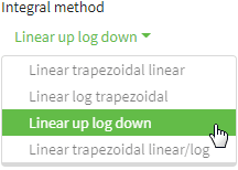
Linear-up / log-down

For an extravascular administration

Straightforward as well. \[\begin{array}{rl}\tag{5} \Delta_t =&t_{i+1}-t_i\\ AUC_i^{i+1}= & \begin{cases} \tfrac{\Delta_t}{2}\,(C_{i+1}+C_i) & \small{\text{if $C_{i+1}\geq C_i$}\textsf{,}}\\ \Delta_t\frac{C_{i+1}\,-\,C_i}{\log_{e}(C_{i+1}/C_i)} & \small{\text{otherwise}\textsf{.}} \end{cases}\\ AUC_{i=1}^{i=n}\;\,= & \sum AUC_i \end{array}\] If subsequent concentrations increase or are equal, the linear trapezoidal $\small{(2)}$ is applied and the log trapezoidal $\small{(3)}$ otherwise.

Visualization

It might not be obvious but all methods interpolate between sampling time points in approximating the integral $\small{\int_{0}^{t}C(t)\,\mathrm{d}t}$. Say, we have a drug with food-induced enterohepatic recycling.

set.seed(123456) # for reproducibility
t    <- c(0, 0.25, 0.5, 1, 1.5, 2, 2.5, 3, 3.5, 4, 5, 6, 9, 12, 16, 24)
# simulated by a one compartment model
C    <- c( 0.00000, 23.14323, 38.84912, 56.09325, 62.65725, 63.99671,
          62.83292, 60.52041, 57.73068, 54.79402, 49.03503, 43.74003,
          30.94365, 21.88070, 13.78398,  5.47017)
CV   <- 0.1
# add lognormal distributed ‘noise’
C    <- rlnorm(n       = length(C),
               meanlog = log(C) - 0.5 * log(CV^2 + 1),
               sdlog   = sqrt(log(CV^2 + 1)))
# increase concentrations at t = 6 and later
C[t >= 6] <- 1.65 * C[t >= 6]
tmax <- t[C == max(C, na.rm = TRUE)]
xlim <- range(t)
ylim <- range(C)
dev.new(width = 3.5, height = 2.6667, record = TRUE)
op   <- par(no.readonly = TRUE)
par(mar = c(3.4, 3.1, 0.1, 0.1), cex.axis = 0.9)
######################
# linear trapezoidal #
######################
# linear scale #
################
plot(t, C, type = "n", xlim = xlim, ylim = ylim,
     xlab = "", ylab = "", axes = FALSE)
mtext(expression(italic(C)*" (m/V)"), 2, line = 2)
grid(nx = NA, ny = NULL)
abline(v = seq(0, 24, 4), lty = 3, col = "lightgrey")
lines(t, C, lwd = 2, col = "blue")
points(t[-1], C[-1], cex = 1.25, pch = 21, col = "blue", bg = "#8080FF80")
axis(1, seq(0, 24, 4))
axis(2, las = 1)
rug(t, ticksize = -0.025)
box()
#############
# log scale #
#############
plot(t[-1], C[-1], type = "n", xlim = xlim, ylim = c(10, ylim[2]),
     log = "y", xlab = "", ylab = "", axes = FALSE)
abline(v = seq(0, 24, 4), lty = 3, col = "lightgrey")
abline(h = axTicks(2), lty = 3, col = "lightgrey")
for (i in 1:(length(t)-1)) {
  tk <- Ck <- NULL # reset segments
  for (k in seq(t[i], t[i+1], length.out = 501)) {
    tk <- c(tk, k)
    Ck <- c(Ck, C[i] + abs((k - t[i]) / (t[i+1] - t[i])) * (C[i+1] - C[i]))
  }
  lines(tk, Ck, col = "blue", lwd = 2)
}
points(t[-1], C[-1], cex = 1.25, pch = 21, col = "blue", bg = "#8080FF80")
axis(1, seq(0, 24, 4))
axis(2, las = 1)
rug(t, ticksize = -0.025)
box()
##########################
# linear log trapezoidal #
##########################
# linear scale #
################
plot(t, C, type = "n", xlim = xlim, ylim = ylim,
     xlab = "", ylab = "", axes = FALSE)
mtext(expression(italic(C)*" (m/V)"), 2, line = 2)
grid(nx = NA, ny = NULL)
abline(v = seq(0, 24, 4), lty = 3, col = "lightgrey")
for (i in 1:(length(t)-1)) {
  if (i <= which(t == tmax)-1) {# linear until tmax
      lines(x = c(t[i], t[i+1]),
            y = c(C[i], C[i+1]),
            col = "blue", lwd = 2)
}else {                      # log afterwards
    tk <- Ck <- NULL # reset segments
    for (k in seq(t[i], t[i+1], length.out = 501)) {
      tk <- c(tk, k)
      Ck <- c(Ck, exp(log(C[i]) + abs((k - t[i]) /
                      (t[i+1] - t[i])) *
                      (log(C[i+1]) - log(C[i]))))
    }
    lines(tk, Ck, col = "magenta", lwd = 2)
  }
}
points(t[-1], C[-1], cex = 1.25, pch = 21, col = "blue", bg = "#8080FF80")
axis(1, seq(0, 24, 4))
axis(2, las = 1)
rug(t, ticksize = -0.025)
box()
#############
# log scale #
#############
plot(t[-1], C[-1], type = "n", xlim = xlim, ylim = c(10, ylim[2]),
     log = "y", xlab = "", ylab = "", axes = FALSE)
abline(v = seq(0, 24, 4), lty = 3, col = "lightgrey")
abline(h = axTicks(2), lty = 3, col = "lightgrey")
lines(c(0, t[2]), c(9, C[2]), col = "blue", lwd = 2)
for (i in 1:(length(t)-1)) {
  if (i <= which(t == tmax)-1) {# linear until tmax
      lines(x = c(t[i], t[i+1]),
            y = c(C[i], C[i+1]),
            col = "blue", lwd = 2)
}else {                      # log afterwards
    tk <- Ck <- NULL # reset segments
    for (k in seq(t[i], t[i+1], length.out = 501)) {
      tk <- c(tk, k)
      Ck <- c(Ck, exp(log(C[i]) + abs((k - t[i]) /
                      (t[i+1] - t[i])) *
                      (log(C[i+1]) - log(C[i]))))
    }
    lines(tk, Ck, col = "magenta", lwd = 2)
  }
}
points(t[-1], C[-1], cex = 1.25, pch = 21, col = "blue", bg = "#8080FF80")
axis(1, seq(0, 24, 4))
axis(2, las = 1)
rug(t, ticksize = -0.025)
box()
####################################
# linear-up / log-down trapezoidal #
####################################
# linear scale #
################
plot(t, C, type = "n", xlim = xlim, ylim = ylim,
     xlab = "", ylab = "", axes = FALSE)
mtext(expression(italic(t)*" (h)"), 1, line = 2.5)
mtext(expression(italic(C)*" (m/V)"), 2, line = 2)
grid(nx = NA, ny = NULL)
abline(v = seq(0, 24, 4), lty = 3, col = "lightgrey")
for (i in 1:(length(t)-1)) {
  if (!is.na(C[i]) & !is.na(C[i+1])) {
    if (C[i+1] >= C[i]) {# increasing (linear)
      lines(x = c(t[i], t[i+1]),
            y = c(C[i], C[i+1]),
            col = "blue", lwd = 2)
  }else {             # decreasing (log)
      tk <- Ck <- NULL # reset segments
      for (k in seq(t[i], t[i+1], length.out = 501)) {
        tk <- c(tk, k)
        Ck <- c(Ck, exp(log(C[i]) + abs((k - t[i]) /
                        (t[i+1] - t[i])) *
                        (log(C[i+1]) - log(C[i]))))
      }
      lines(tk, Ck, col = "magenta", lwd = 2)
    }
  }
}
points(t[-1], C[-1], cex = 1.25, pch = 21, col = "blue", bg = "#8080FF80")
axis(1, seq(0, 24, 4))
axis(2, las = 1)
rug(t, ticksize = -0.025)
box()
#############
# log scale #
#############
plot(t[-1], C[-1], type = "n", xlim = xlim, ylim = c(10, ylim[2]),
     log = "y", xlab = "", ylab = "", axes = FALSE)
mtext(expression(italic(t)*" (h)"), 1, line = 2.5)
abline(v = seq(0, 24, 4), lty = 3, col = "lightgrey")
abline(h = axTicks(2), lty = 3, col = "lightgrey")
lines(c(0, t[2]), c(9, C[2]), col = "blue", lwd = 2)
for (i in 1:(length(t)-1)) {
  if (!is.na(C[i]) & !is.na(C[i+1])) {
    if (C[i+1] >= C[i]) {# increasing (linear)
      lines(x = c(t[i], t[i+1]),
            y = c(C[i], C[i+1]),
            col = "blue", lwd = 2)
  }else {             # decreasing (log)
      tk <- Ck <- NULL # reset segments
      for (k in seq(t[i], t[i+1], length.out = 501)) {
        tk <- c(tk, k)
        Ck <- c(Ck, exp(log(C[i]) + abs((k - t[i]) /
                        (t[i+1] - t[i])) *
                        (log(C[i+1]) - log(C[i]))))
      }
      lines(tk, Ck, col = "magenta", lwd = 2)
    }
  }
}
points(t[-1], C[-1], cex = 1.25, pch = 21, col = "blue", bg = "#8080FF80")
axis(1, seq(0, 24, 4))
axis(2, las = 1)
rug(t, ticksize = -0.025)
box()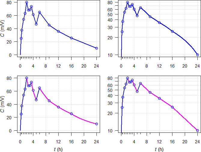

Fig. 3 Interpolations by trapezoidal rules unveiled. Linear sections — and log sections —.
Top panels linear trapezoidal $\small{(2)}$, middle panels linear log trapezoidal $\small{(4)}$,
bottom panels linear-up / log-down trapezoidal rule $\small{(5)}$.
Left panels linear scale, right panels semilogarithmic scale.

Note that using the linear log trapezoidal $\small{(4)}$ would be wrong because it must only be used for an infusion.

No software I’m aware of produces such plots depending on the chosen trapezoidal rule out of the box. Data points are always connected by straight lines, regardless whether a linear or semilogarithmic plot is selected. Producing such plots is moderately difficult in R and would require expertise in commerical software.¹⁰

top of section ↩︎ previous section ↩︎

Data Pretreatment

Don’t import data blindly. Regularly data are obtained from the bioanalytical site containing nonnumeric code(s), e.g., BQL for concentrations below the LLOQ, NR for ‘not reportable’ ones (say, due an interfering peak in chromatography), missing, . in SAS transport files, empty cells in Excel, and NA in R.
This can lead to trouble.

Let’s explore an example (the 66^th simulated profile from below): \[\small{\begin{array}{rc} \hline \text{time} & \text{concentration}\\\hline 0.00 & \text{BQL}\\ 0.25 & \text{BQL}\\ 0.50 & \text{BQL}\\ 0.75 & \text{BQL}\\ 1.00 & 2.386209\\ 1.25 & 3.971026\\ 1.50 & 5.072666\\ 2.00 & 6.461897\\ 2.50 & 5.964697\\ 3.00 & 6.154877\\ 3.50 & 5.742396\\ 4.00 & 4.670705\\ 4.25 & 5.749097\\ 4.50 & 6.376336\\ 4.75 & 6.473850\\ 5.00 & 6.518927\\ 5.25 & 7.197600\\ 5.50 & 7.171507\\ 6.00 & 6.881594\\ 6.50 & 7.345398\\ 7.00 & 7.135752\\ 7.75 & 5.797113\\ 9.00 & 4.520387\\ 12.00 & 3.011526\\ 16.00 & 1.534004\\ 24.00 & 0.369226\\\hline \end{array}}\] If you import this data and press the button,¹¹ likely you will get an $\small{AUC}$ of 77.26565 by the linear trapezoidal rule and 75.64962 by the linear-up / log-down trapezoidal.
But is this correct? Hey, the lag time shows up as zero in the output!

Defining in NCA the lag time as the time point before the time of the first measurable concentration is a convenient consensus. It’s quite obvious that the true one lies somewhere [sic!] between this one and the next. A more realistic approach was suggested¹² but is not implemented in any software.

My trusty Phoenix WinNonlin¹³ dropped all time points where the concentration is BQL, imputed $\small{\text{concentration}=0}$ at $\small{\text{time}=0}$, and informed me in its Core output:¹⁴

Note - the concentration at dose time
was added for extrapolation purposes.

What does that mean? It calculated the first partial $\small{AUC}$ as $\small{(1-0)\times 2.386209/2\approx 1.193105}$. That’s correct numerically though wrong. Well, the software is right but its master, the wetware isn’t. You got what you asked for. Would have been better to RTFM!

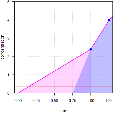
Fig. 4 Imputations unveiled; ● concentrations, — LLOQ.

All ‘hidden’ imputed concentrations are above the LLOQ; the one at 0.75 is with 1.79 already more than five times the LLOQ of 0.34. Of course, that’s nonsense. If that would be true, why couldn’t we measure it?

However, BQL Rules come to the help (see the User’s Guide or the online help for details). A screenshot of the one I use regularly:

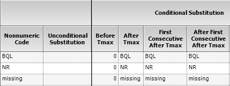
Fig. 5 BQL Rule Set in Phoenix WinNonlin.

Then the leading BQLs are set to zero and the time points 0.25, 0.50, 0.75 kept.

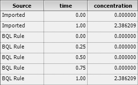
Fig. 6 Naïve import of BQLs vs BQL Rules.

Now we get what we expect: The lag time is reported with 0.75, the $\small{AUC}$ with 76.37082 by the linear trapezoidal and with 74.75479 by the linear-up / log-down trapezoidal.
All is good because the first partial $\small{AUC}$ is correct by $\small{(1-0.75)\times 2.386209/2\approx 0.298276}$.

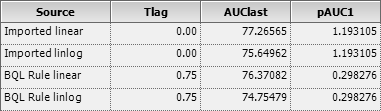
Fig. 7 Congratulations!

I used up to eight significant digits in the example only to allow accurate recalculation. Bioanalytical methods are never – ever! – that precise (more than three significant digits belong to the realm of science fiction).

In the past I experienced questions from assessors when data in full precision (15 digits) were used in calculations but were not reproducible based on the ‘nice’ rounded numbers given in the analytical and statistical reports. This issue will be elaborated in another article.

top of section ↩︎ previous section ↩︎

R Scripts

Trapezoidal rules

A script in Base R to calculate $\small{\textrm{p}AUC_{\Delta\textrm{t}}}$ (partial $\small{AUC}$ within time interval $\small{\Delta \textrm{t}}$) and $\small{AUC_{0-\textrm{t}}}$ by the linear trapezoidal (argument rule = lin) or linear-up / log-down trapezoidal rule (default argument rule = linlog).

Required input are two vectors of times and concentrations. Nonnumeric codes are allowed but must be enclosed in single or double quotes. Missing values have to be specified as NA. By default only $\small{AUC_{0-\textrm{t}_\textrm{last}}\,}$ with the method of calculation in an attribute is returned.

If you want only the numeric result, use calc.AUC(t, C)[["AUClast"]]. When specifying the argument details = TRUE, the entire data frame with the columns t, C, pAUC, AUC is returned.

calc.AUC <- function(t, C, rule = "linlog",
                     digits = 5, details = FALSE) {
  # if nonnumeric codes like BQL or NR are used, they
  # must be enclosed in 'single' or "double" quotes
  if (!length(C) == length(t))
    stop ("Both vectors must have the same number of elements.")
  if (!length(unique(t)) == length(t))
    stop ("Values in t-vector are not unique.")
  if (!rule %in% c("lin", "linlog"))
    stop ("rule must be either \"lin\" or \"linlog\".")
  # convert eventual nonnumerics to NAs
  C    <- unlist(suppressWarnings(lapply(C, as.numeric)))
  tmax <- min(t[C == max(C, na.rm = TRUE)], na.rm = TRUE)
  C[t < tmax & is.na(C)] <- 0    # set NAs prior to tmax to zero
  x    <- NULL
  y    <- data.frame(t = t, C = C, pAUC = 0)
  y    <- y[with(y, order(t)), ] # belt plus suspenders
  NAs  <- which(is.na(C))
  if (sum(NAs) > 0) {            # remove NAs temporarily
    x      <- y[!complete.cases(y), ]
    x$pAUC <- x$AUC <- NA
    y      <- y[complete.cases(y), ]
  }
  for (i in 1:(nrow(y) - 1)) {
    if (rule == "linlog") {
      if (y$C[i+1]  < y$C[i]) {
        y$pAUC[i+1] <- (y$t[i+1] - y$t[i]) * (y$C[i+1] - y$C[i]) /
                       log(y$C[i+1] / y$C[i])
    } else {
        y$pAUC[i+1] <- 0.5 * (y$t[i+1] - y$t[i]) *
                       (y$C[i+1] + y$C[i])
      }
  } else {
      y$pAUC[i+1] <- 0.5 * (y$t[i+1] - y$t[i]) *
                     (y$C[i+1] + y$C[i])
    }
  }
  y$AUC <- cumsum(y$pAUC)
  y     <- rbind(x, y)            # get the NAs back
  y     <- y[with(y, order(t)), ] # sort by time
  if (details) {                  # entire data.frame
    res <- round(y, digits)
} else {                          # only tlast and AUClast
    res <- setNames(as.numeric(round(tail(y[, c(1, 4)], 1), digits)),
                    c("tlast", "AUClast"))
  }
  if (rule == "linlog") {
    attr(res, "trapezoidal rule") <- "linear-up/log-down"
} else {
    attr(res, "trapezoidal rule") <- "linear"
  }
  return(res)
}

previous section ↩︎

Biphasic profiles

To simulate profiles of a biphasic release product. Requires the package truncnorm.¹⁵ Cave: 208 LOC.

Calculates the AUC by the linear and linear-up / log-down trapezoidal rules.
Estimates the % RE (bias) of both methods compared to the theoretical (model’s) AUC.
Plots the profiles in linear and semilogarithmic scale.
Box plots of the % RE of both methods, calculates the difference and its 95% confidence interval based on the Wilcoxon rank sum test.

library(truncnorm)
trap.lin <- function(x, y, first.x, last.x) {
  # linear trapezoidal rule
  pAUC.lin <- 0
  for (i in seq(which(x == first.x), which(x == last.x))) {
    if (x[i] == first.x) { # start triangle
      pAUC.lin <- c(pAUC.lin, 0.5 * (x[i] - x[i-1]) * y[i])
  } else {
      pAUC.lin <- c(pAUC.lin, 0.5 * (x[i] - x[i-1]) * (y[i] + y[i-1]))
    }
  }
  AUC.lin <- cumsum(pAUC.lin)
  return(tail(AUC.lin, 1))
}
trap.linlog <- function(x, y, first.x, last.x) {
  # lin-up/log-down trapezoidal rule
  pAUC.linlog <- 0
  for (i in seq(which(x == first.x), which(x == last.x))) {
    if (x[i] == first.x) {  # start triangle
      pAUC.linlog <- c(pAUC.linlog, 0.5 * (x[i] - x[i-1]) * y[i])
    } else {
      if (y[i] >= y[i-1]) { # linear up
        pAUC.linlog <- c(pAUC.linlog, 0.5 * (x[i] - x[i-1]) * (y[i] + y[i-1]))
    } else {                # log down
        pAUC.linlog <- c(pAUC.linlog,
                         (x[i] - x[i-1]) * (y[i] - y[i-1]) /
                         (log(y[i] / y[i-1])))
      }
    }
  }
  AUC.linlog <- cumsum(pAUC.linlog)
  return(tail(AUC.linlog, 1))
}
set.seed(123456)       # for reproducibility
n       <- 1000        # number of profiles (at least 1)
t       <- c(0,0.25,0.5,0.75,1,1.25,1.5,2,2.5,3,3.5,
             4,4.25,4.5,4.75,5,5.25,5.5,6,6.5,7,7.75,9,12,16,24)
D       <- 100         # guess...
D.f     <- c(0.6, 0.4) # dose fractions of components
# Index ".d" denotes default values, ".c" CV
F.d     <- 0.7         # fraction absorbed (BA)
F.l     <- 0.5         # lower limit
F.u     <- 1           # upper limit
V.d     <- 5           # volume of distribution
V.c     <- 0.50        # CV 50%, lognormal
k01.1.d <- 1.4         # absorption rate constant (1st component)
k01.2.d <- 0.7         # absorption rate constant (2nd component)
k01.c   <- 0.25        # CV 25%, lognormal
k10.d   <- 0.18        # elimination rate constant
k10.c   <- 0.40        # CV 40%, lognormal
tlag1.d <- 0.25        # 1st lag time
tlag1.l <- 5/60        # lower truncation 1
tlag1.u <- 0.75        # upper truncation 1
tlag2.d <- 4           # 2nd lag time
tlag2.l <- 3           # lower truncation 2
tlag.c  <- 0.5         # CV 50%, truncated normal
AErr    <- 0.05        # analytical error CV 5%, lognormal
LLOQ.f  <- 0.05        # fraction of theoretical Cmax

Ct <- function(x, D = D, D.f = D.f, F = F.d, V = V.d,
               k01.1 = k01.1.d, k01.2 = k01.2.d, k10 = k10.d,
               tlag1 = tlag1.d, tlag2 = tlag2.d) {
  C1 <- F.d * D * D.f[1] / V.d * k01.1.d / (k01.1.d - k10.d) *
        (exp(-k10.d * (x - tlag1)) - exp(-k01.1.d * (x - tlag1)))
  C2 <- F.d * D * D.f[2] / V.d * k01.2.d / (k01.2.d - k10.d) *
        (exp(-k10.d * (x - tlag2)) - exp(-k01.2.d * (x - tlag2)))
  C1[C1 < 0] <- 0
  C2[C2 < 0] <- 0
  return(C1 + C2)
}
data  <- data.frame(subject = rep(1:n, each = length(t)), t = t, C = NA)
# individual PK parameters
F     <- runif(n = n, min = F.l, max = F.u)
V     <- rlnorm(n = n, meanlog = log(V.d) - 0.5 * log(V.c^2 + 1),
                sdlog = sqrt(log(V.c^2+1)))
k01.1 <- rlnorm(n = n, meanlog = log(k01.1.d) - 0.5 * log(k01.c^2 + 1),
                sdlog = sqrt(log(k01.c^2 + 1)))
k01.2 <- rlnorm(n = n, meanlog = log(k01.2.d) - 0.5 * log(k01.c^2 + 1),
                sdlog = sqrt(log(k01.c^2 + 1)))
k10   <- rlnorm(n = n, meanlog = log(k10.d) - 0.5 * log(k10.c^2 + 1),
                sdlog = sqrt(log(k10.c^2 + 1)))
tlag1 <- rtruncnorm(n = n, a = tlag1.l, b = tlag1.u,
                    mean = tlag1.d, sd = tlag.c)
tlag2 <- rtruncnorm(n = n, a = tlag2.l, b = Inf,
                    mean = tlag2.d, sd = tlag.c)
x     <- seq(min(t), max(t), length.out = 2501)
# theoretical profile
C.th  <- Ct(x = x, D = D, D.f = D.f, F = F.d, V = V.d,
            k01.1 = k01.1.d, k01.2 = k01.2.d, k10 = k10.d,
            tlag1 = tlag1.d, tlag2 = tlag2.d)
LLOQ  <- LLOQ.f * max(C.th)
# individual profiles
for (i in 1:n) {
  C <- Ct(x = t, D = D, D.f = D.f, F = F[i], V = V[i],
          k01.1 = k01.1[i], k01.2 = k01.2[i], k10 = k10[i],
          tlag1 = tlag1[i], tlag2 = tlag2[i])
  for (j in 1:length(t)) { # analytical error (multiplicative)
    if (j == 1) {
      AErr1 <- rnorm(n = 1, mean = 0, sd = abs(C[j]*AErr))
  } else {
      AErr1 <- c(AErr1, rnorm(n = 1, mean = 0, sd = abs(C[j]*AErr)))
    }
  }
  C <- C + AErr1     # add analytical error
  C[C < LLOQ] <- NA  # assign NAs to Cs below LLOQ
  data$C[data$subject == i] <- C
}
res <- data.frame(subject = 1:n, tlag = NA, tlast = NA, Clast = NA,
                  th = NA, lin = NA, linlog = NA)
# NCA
for (i in 1:n) {
  tmp.t        <- data$t[data$subject == i]
  tmp.C        <- data$C[data$subject == i]
  tfirst       <- t[!is.na(tmp.C)][1]
  tlast        <- rev(tmp.t[!is.na(tmp.C)])[1]
  res$tlag[i]  <- tmp.t[which(tmp.t == tfirst)+1]
  res$tlast[i] <- tlast
  res$Clast[i] <- tmp.C[tmp.t == tlast]
  res$lin[i]   <- trap.lin(tmp.t, tmp.C, tfirst, tlast)
  res$linlog[i] <- trap.linlog(tmp.t, tmp.C, tfirst, tlast)
  compl.t <- x[x >= tfirst & x <= tlast]
  C <- Ct(x = compl.t, D = D, D.f = D.f, F = F[i], V = V[i],
          k01.1 = k01.1[i], k01.2 = k01.2[i], k10 = k10[i],
          tlag1 = tlag1[i], tlag2 = tlag2[i])
  res$th[i] <- 0.5 * sum(diff(compl.t) * (C[-1] + C[-length(C)]))
}
res$RE.lin    <- 100 * (res$lin - res$th) / res$th
res$RE.linlog <- 100 * (res$linlog - res$th) / res$th
# print(res[, c(1:4, 6:7)], row.names = FALSE) # many lines
summary(res[, 8:9])
wt <- wilcox.test(res$RE.lin, res$RE.linlog, conf.int = TRUE)

# spaghetti plot
C <- Ct(x = x, D = D, D.f = D.f, F = F.d, V = V.d,
        k01.1 = k01.1.d, k01.2 = k01.2.d, k10 = k10.d,
        tlag1 = tlag1.d, tlag2 = tlag2.d)
C[C == 0] <- NA
log.plot <- FALSE
if (log.plot) {
  log.y <- "y"
  ylim <- c(LLOQ * 0.9, 1.2 * max(data$C, na.rm = TRUE))
} else {
  log.y <- ""
  ylim <- c(0, 1.04 * max(data$C, na.rm = TRUE))
}
dev.new(width = 4.5, height = 4.5, record = TRUE)
op <- par(no.readonly = TRUE)
par(mar = c(4, 2.9, 0.2, 0.1), cex.axis = 0.9,
    xaxs = "r", yaxs = "i")
plot(x, C, type = "n", axes = FALSE, ylim = ylim, log = log.y,
     xlab = "time", ylab = "")
mtext("concentration", 2, line = 2)
axis(1, at = c(seq(0, 6, 2), c(9, 12, 16, 24)))
axis(2, las = 1)
abline(h = LLOQ, col = "red")
rug(t, ticksize = -0.015)
for (i in 1:n) {
  tmp.C  <- data$C[data$subject == i]
  tfirst <- t[!is.na(tmp.C)][1]      # 1st C >= LLOQ
  tlast  <- rev(t[!is.na(tmp.C)])[1] # last C >= LLOQ
  for (j in 1:(length(t)-1)) {
    if (!is.na(tmp.C[j]) & !is.na(tmp.C[j+1])) {
      if (tmp.C[j+1] >= tmp.C[j]) {  # up (linear)
        lines(x = c(t[j], t[j+1]),
              y = c(tmp.C[j], tmp.C[j+1]), col = "#0000FF80") 
    } else {                         # down (linlog)
        tk <- NULL
        Ck <- NULL
        for (k in seq(t[j], t[j+1], length.out = 100)) {
          tk <- c(tk, k)
          Ck <- c(Ck, exp(log(tmp.C[j]) + abs((k - t[j]) / (t[j+1] - t[j])) *
                         (log(tmp.C[j+1]) - log(tmp.C[j]))))
        }
        lines(tk, Ck, col = "#FF00FF80")
      }
    }
  }
}
lines(x, C, type = "l", lwd = 3, col = "#00000080")
leg <- c(expression(C[t[italic(i)]]>=C[t[italic(i)-1]]*" (linear up)"),
         expression(C[t[italic(i)]]>=C[t[italic(i)-1]]*" (log down)"),
         "theoretical profile", "LLOQ")
legend("topright", box.lty = 0, y.intersp = 1.2, lwd = c(1, 1, 3, 1),
       col = c("#0000FF80", "#FF00FF80", "#00000080", "red"),
       legend = leg, seg.len = 2.5)
box()

# box plots
ylim <- 1.04 * c(-1, +1) * max(abs(range(res[, 8:9])))
op <- par(no.readonly = TRUE)
par(mar = c(0, 2.9, 0, 0), cex.axis = 0.9)
plot(c(0.5, 2.5), c(0, 0), ylim = ylim, type = "n", axes = FALSE,
     xlab = "", ylab = "")
abline(h=0, lty=3)
boxplot(res$RE.lin, res$RE.linlog, boxwex = 0.35, notch = TRUE,
        notch.frac = 0.6, ylim = ylim, names = "", ylab = "",
        main = "", axes = FALSE, col = "bisque", outcol = "red", add = TRUE)
axis(2, las = 1)
mtext("linear", at = 1, 1, line = -1.1)
mtext("lin-up / log-down", at = 2, 1, line = -1.1)
mtext("relative error (%)", 2, line = 2)
wilc.diff <- paste0("\u2206 ", sprintf("%+.3f", wt$estimate), "\n95% CI ",
                    sprintf("(%+.3f", wt$conf.int[1]), ", ",
                    sprintf("%+.3f)", wt$conf.int[2]))
text(x = 1.5, y = min(res[, 8:9]), labels = wilc.diff, cex = 0.9)
par(op)

previous section ↩︎

One-compartment model

A one-compartment model (first order absorption and elimination) with rich and sparse sampling.
Cave: 222 LOC.

Calculates the AUC by the linear and linear-up / log-down trapezoidal rules.
Estimates the bias compared to the theoretical (model’s) AUC.
Plots of the profile in linear scale.

rich.sparse <- function() {
  one.comp <- function(f, D, V, k01, k10, t, t.last) { # no lagtime
    if (!isTRUE(all.equal(k01, k10))) { # common: k01 ≠ k10
      C    <- f * D * k01 / (V * (k01 - k10)) *
              (exp(-k10 * t) - exp(-k01 * t))
      tmax <- log(k01 / k10) / (k01 - k10)
      Cmax <- f * D * k01 / (V * (k01 - k10)) *
              (exp(-k10 * tmax) - exp(-k01 * tmax))
      AUC  <- f * D / V / k10
      x    <- micro.macro(f, D, V, k01, k10)
      AUCt <- (x$C[["A"]] - x$C[["A"]] * exp(-x$E[["alpha"]] * t.last)) /
              x$E[["alpha"]] +
              (x$C[["B"]] - x$C[["B"]] * exp(-x$E[["beta"]] * t.last)) /
              x$E[["beta"]]
  } else {                              # flip-flop
      k    <- k10
      C    <- f * D / V * k * t * exp(-k * t)
      tmax <- 1 / k
      Cmax <- f * D / V * k * tmax * exp(-k * tmax)
      AUC  <- f * D / V / k
      AUCt <- NA # no idea
    }
    res <- list(C = C, tmax = tmax, Cmax = Cmax, AUC = AUC, AUCt = AUCt)
    return(res)
  }
  micro.macro <- function(f, D, V, k01, k10) {
    # Coefficients (C) and exponents (E)
    C <- f * D * k01 / (V * (k01 - k10))
    C <- setNames(c(-C, +C), c("A", "B"))
    E <- setNames(c(k01, k10), c("alpha", "beta"))
    macro <- list(C = C, E = E)
    return(macro)
  }
  NCA <- function(t, C, t.first, t.last, lambda.z) {
    pAUC.linlog <- 0
    for (i in seq(which(t == t.first), which(t == t.last))) {
      if (t[i] == t.first) { # first triangle if 0
        pAUC.linlog <- c(pAUC.linlog, 0.5 * (t[i] - t[i-1]) * C[i])
      } else {
        if (C[i] >= C[i-1]) { # linear up
          pAUC.linlog <- c(pAUC.linlog, 0.5*(t[i] - t[i-1]) * (C[i] + C[i-1]))
      } else {                # log down
          pAUC.linlog <- c(pAUC.linlog,
                           (t[i] - t[i-1]) * (C[i] - C[i-1]) /
                           (log(C[i] / C[i-1])))
        }
      }
    }
    AUC.linlog <- tail(cumsum(pAUC.linlog), 1)
    AUC.inf    <- AUC.linlog + tail(C, 1) / lambda.z
    Cmax       <- max(C)
    tmax       <- t[C == Cmax]
    res        <- list(AUCt = AUC.linlog, AUCinf = AUC.inf,
                       Cmax = Cmax, tmax = tmax)
    return(res)
  }
  lz <- function(t, C) {
    m <- lm(log(C) ~ t)
    return(-coef(m)[[2]])
  }
  f           <- 2 / 3
  D           <- 400
  V           <- 3.49
  t12.01      <- 1
  t12.10      <- 6
  k01         <- log(2) / t12.01
  k10         <- log(2) / t12.10
  t           <- seq(0, 24, length.out = 501)
  rich.smpl   <- c(0, 0.25, 0.5, 1, 1.5, 2, 2.5, 3, 3.5, 4, 5, 6, 9, 12, 16, 24)
  sparse.smpl <- c(0, 0.5, 1.5, 2.5, 3.5, 5, 9, 12, 24)
  model       <- one.comp(f, D, V, k01, k10, t, 24)
  rich        <- one.comp(f, D, V, k01, k10, rich.smpl, 24)
  sparse      <- one.comp(f, D, V, k01, k10, sparse.smpl, 24)
  rich.NCA    <- NCA(rich.smpl, rich$C, 0, 24,
                     lz(tail(rich.smpl, 3), tail(rich$C, 3)))
  sparse.NCA  <- NCA(sparse.smpl, sparse$C, 0, 24,
                     lz(tail(sparse.smpl, 3), tail(sparse$C, 3)))
  result      <- data.frame(method = c("exact (from model) ",
                                       "NCA rich sampling  ",
                                       "NCA sparse sampling"),
                            AUCt = sprintf("%.2f",
                                           c(model$AUCt,
                                             rich.NCA$AUCt,
                                             sparse.NCA$AUCt)),
                            AUCinf = sprintf("%.2f",
                                             c(model$AUC,
                                               rich.NCA$AUCinf,
                                               sparse.NCA$AUCinf)),
                            Cmax = sprintf("%.3f",
                                           c(model$Cmax,
                                             rich.NCA$Cmax,
                                             sparse.NCA$Cmax)),
                            tmax = sprintf("%.3f",
                                           c(model$tmax,
                                             rich.NCA$tmax,
                                             sparse.NCA$tmax)))
  bias        <- data.frame(sampling = c("rich    ", "sparse  "),
                            AUCt = c(sprintf("%+.3f%%",
                                     100 * (rich.NCA$AUCt - model$AUCt) /
                                     model$AUCt),
                                     sprintf("%+.3f%%",
                                     100 * (sparse.NCA$AUCt - model$AUCt) /
                                     model$AUCt)),
                            AUCinf = c(sprintf("%+.3f%%",
                                       100 * (rich.NCA$AUCinf - model$AUC) /
                                       model$AUC),
                                       sprintf("%+.3f%%",
                                       100 * (sparse.NCA$AUCinf - model$AUC) /
                                       model$AUC)),
                            Cmax = c(sprintf("%+.3f%%",
                                     100 * (rich.NCA$Cmax - model$Cmax) /
                                     model$Cmax),
                                     sprintf("%+.3f%%",
                                     100 * (sparse.NCA$Cmax - model$Cmax) /
                                     model$Cmax)),
                            tmax = c(sprintf("%+.3f", rich.NCA$tmax-model$tmax),
                                     sprintf("%+.3f", sparse.NCA$tmax-model$tmax)))
  txt         <- "Bias (NCA results compared to the model)\n"
  xlim        <- range(t)
  ylim        <- range(model$C)
  dev.new(width = 4.5, height = 4.5)
  op          <- par(no.readonly = TRUE)
  par(mar = c(3.4, 3.1, 0, 0.1), cex.axis = 0.9)
  plot(t, model$C, type = "n", ylim = c(0, model$Cmax),
       xlab = "", ylab = "", axes = FALSE)
  mtext(expression(italic(t)*" (h)"), 1, line = 2.5)
  mtext(expression(italic(C)*" (m/V)"), 2, line = 2)
  grid(nx = NA, ny = NULL)
  abline(v = seq(0, 24, 4), lty = 3, col = "lightgrey")
  polygon(c(t, rev(t)), c(rep(0, length(model$C)), rev(model$C)),
          border = "#87CEFA80", col = "#87CEFA80")
  for (i in 1:(length(rich.smpl)-1)) {
    if (!is.na(rich$C[i]) & !is.na(rich$C[i+1])) {
      if (rich$C[i+1] >= rich$C[i]) { # up (lin)
        lines(x = c(rich.smpl[i], rich.smpl[i+1]),
              y = c(rich$C[i], rich$C[i+1]),
              col = "#0000FF80", lwd = 2)
    } else {                          # down (log)
        tk <- NULL
        Ck <- NULL
        for (k in seq(rich.smpl[i], rich.smpl[i+1], length.out = 201)) {
          tk <- c(tk, k)
          Ck <- c(Ck, exp(log(rich$C[i]) + abs((k - rich.smpl[i])/
                         (rich.smpl[i+1] - rich.smpl[i])) *
                         (log(rich$C[i+1]) - log(rich$C[i]))))
        }
        lines(tk, Ck, col = "#0000FF80", lwd = 2)
      }
    }
  }
  for (i in 1:(length(sparse.smpl)-1)) {
    if (!is.na(sparse$C[i]) & !is.na(sparse$C[i+1])) {
      if (sparse$C[i+1] >= sparse$C[i]) { # up (lin)
        lines(x = c(sparse.smpl[i], sparse.smpl[i+1]),
              y = c(sparse$C[i], sparse$C[i+1]),
              col = "#FF000080", lwd = 2)
    } else {                              # down (log)
        tk <- NULL
        Ck <- NULL
        for (k in seq(sparse.smpl[i], sparse.smpl[i+1], length.out = 201)) {
          tk <- c(tk, k)
          Ck <- c(Ck, exp(log(sparse$C[i]) + abs((k-sparse.smpl[i]) /
                         (sparse.smpl[i+1] - sparse.smpl[i])) *
                         (log(sparse$C[i+1]) - log(sparse$C[i]))))
        }
        lines(tk, Ck, col = "#FF000080", lwd = 2)
      }
    }
  }
  axis(1, seq(0, 24, 4))
  axis(2, las = 1)
  box()
  plotdim     <- par("plt") # coordinates for inset plot
  xleft       <- plotdim[2] - (plotdim[2] - plotdim[1]) * 0.55
  xright      <- plotdim[2]
  ybottom     <- plotdim[4] - (plotdim[4] - plotdim[3]) * 0.4
  ytop        <- plotdim[4]
  par(fig = c(xleft, xright, ybottom, ytop), mar = rep(0, 4),
      cex.axis = 0.8, new = TRUE)
  plot(t[t <= model$tmax], model$C[t <= model$tmax],
       type = "n", ylim = c(0, model$Cmax),
       xlab = "", ylab = "", axes = FALSE)
  rect(0, 0, t[t <= model$tmax], model$Cmax, col = "white", border = NA)
  grid(nx = NA, ny = NULL)
  abline(v = 0:3, lty = 3, col = "lightgrey")
  polygon(c(t[t <= model$tmax], rev(t[t <= model$tmax])),
          c(rep(0, length(model$C[t <= model$tmax])),
            rev(model$C[t <= model$tmax])),
          border = "#87CEFA80", col = "#87CEFA80")
  for (i in 1:(length(rich.smpl)-1)) {
    if (!is.na(rich$C[i]) & !is.na(rich$C[i+1])) {
      if (rich$C[i+1] >= rich$C[i]) { # up (linear)
        lines(x = c(rich.smpl[i], rich.smpl[i+1]),
              y = c(rich$C[i], rich$C[i+1]),
              col = "#0000FF80", lwd = 2)
    } else {                          # down (log)
        tk <- NULL
        Ck <- NULL
        for (k in seq(rich.smpl[i], rich.smpl[i+1], length.out = 201)) {
          tk <- c(tk, k)
          Ck <- c(Ck, exp(log(rich$C[i]) + abs((k - rich.smpl[i]) /
                         (rich.smpl[i+1] - rich.smpl[i])) *
                         (log(rich$C[i+1]) - log(rich$C[i]))))
        }
        lines(tk, Ck, col = "#0000FF80", lwd = 2)
      }
    }
  }
  for (i in 1:(length(sparse.smpl)-1)) {
    if (!is.na(sparse$C[i]) & !is.na(sparse$C[i+1])) {
      if (sparse$C[i+1] >= sparse$C[i]) { # up (lin)
        lines(x = c(sparse.smpl[i], sparse.smpl[i+1]),
              y = c(sparse$C[i], sparse$C[i+1]),
              col = "#FF000080", lwd = 2)
    } else {                              # down (log)
        tk <- NULL
        Ck <- NULL
        for (k in seq(sparse.smpl[i], sparse.smpl[i+1], length.out = 201)) {
          tk <- c(tk, k)
          Ck <- c(Ck, exp(log(sparse$C[i]) + abs((k-sparse.smpl[i]) /
                         (sparse.smpl[i+1] - sparse.smpl[i])) *
                         (log(sparse$C[i+1]) - log(sparse$C[i]))))
        }
        lines(tk, Ck, col = "#FF000080", lwd = 2)
      }
    }
  }
  axis(1, 0:3)
  box()
  par(op)
  print(result, row.names = FALSE); cat(txt); print(bias, row.names = FALSE)
}

previous section ↩︎

Examples

Missing Values

The positive bias of the linear trapezoidal rule gets especially nasty if values are missing within the profile (so-called ‘embedded missings’).
Here I removed the 16 h value of the first simulated biphasic profile (see below).

# you have to run the simulation script before
t.full <- data$t[data$subject == 1]
C.full <- data$C[data$subject == 1]
C.miss <- C.full[-which(t.full == 16)]
t.miss <- t.full[-which(t.full == 16)]
tfirst <- t[!is.na(C.full)][1]
tlast  <- rev(t.full[!is.na(C.full)])[1]
comp   <- data.frame(dataset = c("full", "16 h missing"),
                     lin = NA, linlog = NA)
comp$lin[1]    <- trap.lin(t.full, C.full, tfirst, tlast)
comp$linlog[1] <- trap.linlog(t.full, C.full, tfirst, tlast)
comp$lin[2]    <- trap.lin(t.miss, C.miss, tfirst, tlast)
comp$linlog[2] <- trap.linlog(t.miss, C.miss, tfirst, tlast)
print(comp, row.names = FALSE)
dev.new(width = 4.5, height = 4.5)
op <- par(no.readonly = TRUE)
par(mar = c(4, 2.9, 0.2, 0.1), cex.axis = 0.9,
    xaxs = "r", yaxs = "i")
plot(t.miss, C.miss, type="n", axes = FALSE,
     ylim = c(0, 1.04*max(data$C, na.rm = TRUE)),
     xlab = "time", ylab = "")
mtext("concentration", 2, line = 2)
axis(1, at = c(seq(0, 6, 2), c(9, 12, 16, 24)))
axis(2, las = 1)
abline(h = LLOQ, col = "red")
rug(t, ticksize = -0.015)
points(16, C.full[which(t.full == 16)], pch = 19,
       cex = 1.25, col = "red") # the ‘missing’ one
# linear
lines(t.miss, C.miss, col = "#FF00FF80", lwd = 2)
# lin-up / log-down
for (i in 1:(length(t.miss)-1)) {
  if (!is.na(C.miss[i]) & !is.na(C.miss[i+1])) {
    if (C.miss[i+1] >= C.miss[i]) { # up (linear)
      lines(x = c(t.miss[i], t.miss[i+1]),
            y = c(C.miss[i], C.miss[i+1]),
            col = "#0000FF80", lwd = 2)
  } else {                         # down (linlog)
      tk <- NULL
      Ck <- NULL
      for (k in seq(t[i], t.miss[i+1], length.out = 200)) {
        tk <- c(tk, k)
        Ck <- c(Ck, exp(log(C.miss[i]) + abs((k-t.miss[i]) /
                       (t.miss[i+1] - t.miss[i])) *
                       (log(C.miss[i+1]) - log(C.miss[i]))))
      }
      lines(tk, Ck, col = "#0000FF80", lwd = 2)
    }
  }
}
legend("topright", box.lty = 0, y.intersp = 1.2, lwd = c(2, 2, 1),
       col = c("#FF00FF80", "#0000FF80", "red"), seg.len = 2.5,
       legend = c("linear", "lin-up / log-down", "LLOQ"))
box()
par(op)

#       dataset      lin   linlog
#          full 77.42499 75.71357
#  16 h missing 82.97551 76.56601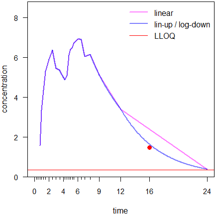

Fig. 8 First simulated profile (● is the ‘missing’ value).

Connecting the 12 and 24 hours data by a straight line in the linear trapezoidal fires back (bias of $\small{AUC_{0-t_\textrm{last}}}$ +7.2%). The linear-up / log-down is much less affected (bias of $\small{AUC_{0-t_\textrm{last}}}$ +1.1%).

Hence, if the linear trapezoidal is used, in a comparative BA study missing values bias the T/R-ratio.

However, as seen in Fig. 1 and Fig. 2, the more similar two concentrations (in the Figures $\small{a}$ and $\small{b}$), the more similar the areas obtained by the linear and linear-up / log-down trapezoidal. Or the other way round: The narrower the sampling interval, the smaller the difference obtained by the two methods. Hence, if the linear trapezoidal is used, missings in a section of the profile with rich sampling hurt less than in a section with wide intervals.

I also misused the example above and removed the concentrations at 9 and 16 hours.

t     <- c(0.00, 0.25, 0.50, 0.75, 1.00,  1.25,  1.50,  2.00, 2.50,
           3.00, 3.50, 4.00, 4.25, 4.50,  4.75,  5.00,  5.25, 5.50,
           6.00, 6.50, 7.00, 7.75, 9.00, 12.00, 16.00, 24.00)
C <- M <- c("BQL", "BQL", "BQL", "BQL",
            2.386209, 3.971026, 5.072666, 6.461897, 5.964697, 6.154877,
            5.742396, 4.670705, 5.749097, 6.376336, 6.473850, 6.518927,
            7.197600, 7.171507, 6.881594, 7.345398, 7.135752, 5.797113,
            4.520387, 3.011526, 1.534004, 0.369226)
M[t %in% c(9, 16)] <- NA
res <- data.frame(data    = c(rep("complete", 2), rep("missings", 2)),
                  method  = rep(c("lin", "linlog"), 2),
                  AUClast = c(calc.AUC(t, C, method = "lin")[["AUClast"]],
                              calc.AUC(t, C, method = "linlog")[["AUClast"]],
                              calc.AUC(t, M, method = "lin")[["AUClast"]],
                              calc.AUC(t, M, method = "linlog")[["AUClast"]]))
print(res, row.names = FALSE, right = FALSE)

#  data     method AUClast 
#  complete lin    76.37082
#  complete linlog 74.75479
#  missings lin    80.92340
#  missings linlog 75.07470

As usual we see the positive bias of the linear trapezoidal. If we compare the data set with missings to the complete one, we see that with the linear trapezoidal the result changed by +5.96% but with the linear-up / log-down only by +0.43%. Convinced?

top of section ↩︎ previous section ↩︎

Simulations

I’ve chosen a difficult one. A biphasic release formulation, one compartment model, PK-parameters: $\small{D=100}$, dose fractions of the IR and DR components $\small{\left\{0.6,0.4\right\}}$, fraction absorbed $\small{f=0.70}$, volume of distribution $\small{V=5}$, absorption rate constants of the components $\small{k_{\,01.\textrm{IR}}=1.4\,\textrm{h}^{-1}}$, $\small{k_{\,01.\textrm{DR}}=0.7\,\textrm{h}^{-1}}$, lag times of the components $\small{tlag_{\,01.\textrm{IR}}=25\,\textrm{min}}$, $\small{tlag_{\,01.\textrm{DR}}=4\,\textrm{h}}$, elimination rate constant $\small{k_{\,10}=0.18\,\textrm{h}^{-1}}$.
The sampling schedule was $\small{0}$, $\small{0.25}$, $\small{0.5}$, $\small{0.75}$, $\small{1}$, $\small{1.25}$, $\small{1.5}$, $\small{2}$, $\small{2.5}$, $\small{3}$, $\small{3.5}$, $\small{4}$, $\small{4.25}$, $\small{4.5}$, $\small{4.75}$, $\small{5}$, $\small{5.25}$, $\small{5.5}$, $\small{6}$, $\small{6.5}$, $\small{7}$, $\small{7.75}$, $\small{9}$, $\small{12}$, $\small{16}$, and $\small{24}$ hours in order to get reliable estimates of both peaks.
Error distributions were uniform for $\small{f}$ $\small{(0.5-1)}$, log-normal for $\small{V}$ $\small{(CV=50\%)}$, $\small{k_{\,01}}$ $\small{(CV=25\%)}$, $\small{k_{\,10}}$ $\small{(CV=40\%)}$, and truncated normal for $\small{tlag_{\,01.\textrm{IR}}}$ $\small{(5-45\,\text{min},\,CV=50\%)}$, $\small{tlag_{\,02.\textrm{DR}}}$ $\small{(\geq3\,\text{h},\,CV=50\%)}$. Analytical error was log-normal with $\small{CV=5\%}$ of the simulated concentration.

1,000 simulated profiles, the LLOQ was set to 5% of the theoretical $\small{C_\textrm{max}}$, i.e., simulated concentrations below the LLOQ were forced to NA. $\small{AUC_{0-t_{\textrm{last}}}}$ was calculated by both methods and compared to the true one (without analytical error).

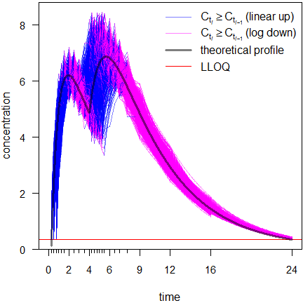
Fig. 9 Linear scale.

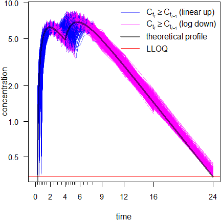
Fig. 10 Semilogarithmic scale.

All results agreed with Phoenix WinNonlin.
Lag times were in 230 profiles 0.5 h, in 407 0.75 h, in 337 1 h, and in 26 1.25 h. In 493 profiles $\small{t_{\textrm{last}}}$ was at 16 hours and in 507 at 24 hours.

After 16 hours the profiles may give a false impression. Any kind of average plot would be positively biased. This will be elaborated in another article.

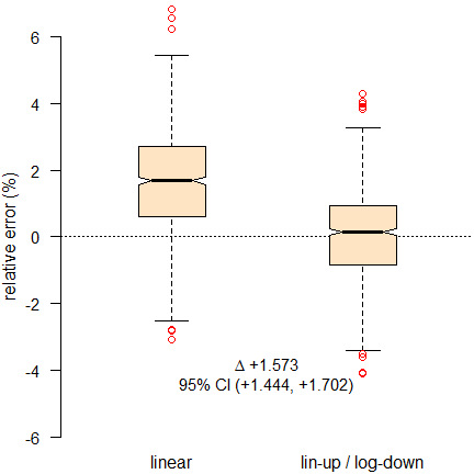
Fig. 11 Relative errors of $\small{AUC_{0-t_\textrm{last}}\,}$.

The linear and linear-up / log-down trapezoidal rules (compared to the theoretical $\small{AUC}$ of profiles without analytical error) clearly show the positive bias of the former and that it performs significantly worse than the latter.
The slight bias in the linear-up / log-down trapezoidal is due to the linear part. Better methods to estimate the absorption phase(s) were proposed¹⁶ but are currently not implemented in any software. For details see below.

Hence, there is no good reason to stick to the linear trapezoidal rule any more.

top of section ↩︎ previous section ↩︎

Implementations

The linear-up / log-down trapezoidal rule is implemented for decades (‼) in standard software.¹⁷ ¹⁸

Phoenix WinNonlin

It’s just one click in the NCA Options (see the online help for details). Don’t tell me that’s complicated.

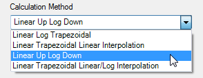
Fig. 12 NCA Options in Phoenix WinNonlin.

PKanalix

Available in the NCA Settings.¹⁹

Fig. 13 NCA Calculations in PKanalix.

R Packages

In bear²⁰ ²¹ the linear-up / log-down trapezoidal rule is the default since June 2013. THX to Yung-jin!

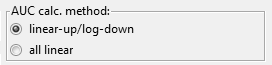
Fig. 14 AUC calculation in bear.

In PKNCA,²² ²³ ncappc,²⁴ NonCompart,²⁵ ncar,²⁶ pkr,²⁷ and qpNCA²⁸ both are supported. Whilst in the first two the linear-up / log-down trapezoidal rule is the default, in the others it is the linear trapezoidal rule.
Regrettably, ubiquity²⁹ ³⁰ ³¹ and PK³² ³³ support only the linear trapezoidal.

A simple example with $\small{t=\left\{0, 0.25, 1, 2, 4, 8\right\}}$ and $\small{C=\left\{0, 13.38, 25, 18.75, 5.86, 0.39\right\}}$ evaluated with my script in Base R (no package required).

t <- c(0.00,  0.25,  1.00,  2.00, 4.00, 8.00)
C <- c(0.00, 13.38, 25.00, 18.75, 5.86, 0.39)
print(calc.AUC(t, C, details = TRUE), row.names = FALSE)

#     t     C     pAUC      AUC
#  0.00  0.00  0.00000  0.00000
#  0.25 13.38  1.67250  1.67250
#  1.00 25.00 14.39250 16.06500
#  2.00 18.75 21.72537 37.79037
#  4.00  5.86 22.16597 59.95634
#  8.00  0.39  8.07452 68.03086

This time the example data with BQLs from above. By default only the relevant information, i.e., the time point of the last measurable concentration, the associated $\small{AUC_{0-t_\textrm{last}}\,}$, and the method of its calculation is shown:

t <- c(0.00, 0.25, 0.50, 0.75, 1.00,  1.25,  1.50,  2.00, 2.50,
       3.00, 3.50, 4.00, 4.25, 4.50,  4.75,  5.00,  5.25, 5.50,
       6.00, 6.50, 7.00, 7.75, 9.00, 12.00, 16.00, 24.00)
C <- c("BQL", "BQL", "BQL", "BQL",
       2.386209, 3.971026, 5.072666, 6.461897, 5.964697, 6.154877,
       5.742396, 4.670705, 5.749097, 6.376336, 6.473850, 6.518927,
       7.197600, 7.171507, 6.881594, 7.345398, 7.135752, 5.797113,
       4.520387, 3.011526, 1.534004, 0.369226)
calc.AUC(t, C) # all defaults used

#    tlast  AUClast 
# 24.00000 74.75479 
# attr(,"trapezoidal rule")
# [1] "linear-up/log-down"

To show only the numeric result, use calc.AUC(t, C)[["AUClast"]].

calc.AUC(t, C)[["AUClast"]]

# [1] 74.75479

Julia Libraries

In the Clinical Trial Utilities³⁴ both the linear and the linear-up / log-down trapezoidal rules are implemented, where the linear trapezoidal rule is the default. It was cross-validated against Phoenix WinNonlin.
In Pumas³⁵ both are implemented, where the linear trapezoidal rule is the default as well.³⁶ It was cross-validated against Phoenix WinNonlin and PKNCA.

Spreadsheets

Although I definitely don’t recommend it, doable. The simple example from above:

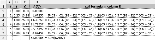
Fig. 15 Linear-up / log-down rule in a spreadsheet.

Good luck if you have rich sampling and a lot of subjects… Furthermore, a proper handling of missing values with the formula interface would be a nightmare. Macros are likely a better approach.

Interlude: Increasing concentrations

Since Purves’ method¹⁶ is not implemented in any software, we’ll make do with what we have. Although the linear log and linear-up / log-down trapezoidal rules perform extremely well for decreasing concentrations, there is still a negative bias in the increasing sections of the profile.

An example of a simple one-compartment model with rich (16 time points) and sparse (nine time points) sampling:

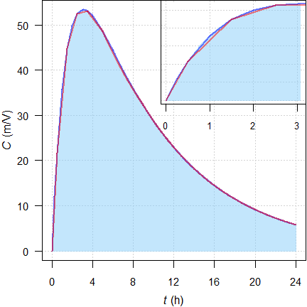
Fig. 16 Rich (—) and sparse (—) sampling. Shaded area is the model.
Early section of the profile in the inset.

rich.sparse()

#               method   AUCt AUCinf   Cmax  tmax
#  exact (from model)  611.80 661.41 53.397 3.102
#  NCA rich sampling   610.25 659.89 53.374 3.000
#  NCA sparse sampling 606.28 656.01 53.092 3.500
# Bias (NCA results compared to the model)
#  sampling    AUCt  AUCinf    Cmax   tmax
#  rich     -0.253% -0.229% -0.043% -0.102
#  sparse   -0.902% -0.816% -0.571% +0.398

Since in the early section (up to the inflection point at $\small{2\times t_\textrm{max}}$³⁷) the profile is concave, the $\small{AUC}$ is underestimated. However, the bias decreases if we extrapolate to infinity.
Naturally, we fare better with rich sampling.

An example of a long constant-rate infusion, linear log trapezoidal:

C.inf <- function(D, V, k10, loi, t) {
  # one compartment model, constant rate infusion
  # zero order input [mass / time]
  r   <- D / loi
  # concentration during infusion
  C.1 <- r / (V * k10) * (1 - exp(-k10 * t[t <= loi]))
  # concentration after end of infusion
  C.2 <- tail(C.1, 1) * exp(-k10 * (t[t > loi] - loi))
  # combine both
  C   <- c(C.1, C.2)
  return(C)
}
D     <- 250 # dose
V     <- 2   # volume of distribution
loi   <- 4   # length of infusion
t.el  <- 6   # elimination half life
k10   <- log(2) / t.el
t     <- c(0, 2, 4, 5)
C     <- C.inf(D, V, k10, loi, t)
tmax  <- t[C == max(C)]
t.mod <- seq(min(t), max(t), length.out = 501)
C.mod <- C.inf(D, V, k10, loi, t.mod)
dev.new(width = 4.5, height = 4.5)
op    <- par(no.readonly = TRUE)
par(mar = c(3.4, 3.1, 0, 0), cex.axis = 0.9)
plot(t, C, type = "n", xlab = "", ylab = "", axes = FALSE)
mtext(expression(italic(t)*" (h)"), 1, line = 2.5)
mtext(expression(italic(C)*" (m/V)"), 2, line = 2)
grid()
lines(t.mod, C.mod, col = "red", lwd = 2)
for (i in 1:(length(t)-1)) {
  if (i <= which(t == tmax)-1) { # linear until tmax
      lines(x = c(t[i], t[i+1]),
            y = c(C[i], C[i+1]),
            col = "blue", lwd = 2)
} else {                        # log afterwards
    tk <- Ck <- NULL # reset segments
    for (k in seq(t[i], t[i+1], length.out = 501)) {
      tk <- c(tk, k)
      Ck <- c(Ck, exp(log(C[i]) + abs((k - t[i]) /
                      (t[i+1] - t[i])) *
                      (log(C[i+1]) - log(C[i]))))
    }
    lines(tk, Ck, col = "magenta", lwd = 2)
  }
}
points(t[-1], C[-1], cex = 1.25, pch = 21, col = "blue", bg = "#8080FF80")
axis(1)
axis(2, las = 1)
box()
par(op)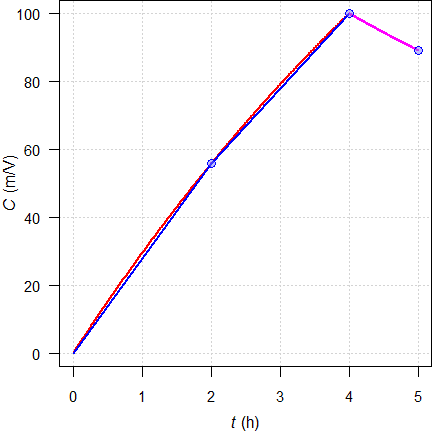

Fig. 17 Theoretical concentrations (—);
linear interpolation for $\small{t\leq t_\text{max}}$ (—), logarithmic for $\small{t>t_\text{max}}$ (—).

To counteract a bias due to the concave shape of the profile during zero order input, sampling before the end of infusion is recommended.

top of section ↩︎ previous section ↩︎

Recommendation

Always state³⁸ in the $\small{\frac{\textsf{protocol}}{\textsf{report}}}$ which trapezoidal rule you $\small{\frac{\textsf{will use}}{\textsf{used}}}$ (see also the article about extrapolation to infinity).
It supports assessors³⁹ to verify your results. Referring only to an SOP is not a good idea because it not accessible to regulators.

Nowadays, the linear trapezoidal rule is mainly of historic interest. Under the premise of linear³ PK it should be thrown into the pharmacometric waste container.
🚮

Abandon calculating the AUC by the linear trapezoidal rule. Your results will inevitably be biased and lead in trouble, especially if values are missing.

If your SOP still calls for the linear trapezoidal rule, it is time for an update based on science, rather following outdated customs.

top of section ↩︎ previous section ↩︎

Postscript

As an instructor, it is fine to present the linear trapezoidal rule in its historic context at the beginning of the pharmacology curriculum. Heck, Yeh and Kwan⁶ wrote about the bias of the linear trapezoidal already 45 years ago. For a good while we are living in the 21^st century!

Maybe you have the classic⁴⁰ on your bookshelf.

“[…] the log trapezoidal method can be be used advantageously in combination with a second method, such as the linear trapezoidal rule, to yield optimal estimates.
Gibaldi and Perrier (1982)⁴⁰

For the time being, the linear-up / log-down trapezoidal rule should be elaborated⁴¹ ⁴² ⁴³ and suggested to students.

top of section ↩︎ previous section ↩︎

Acknowledgments

Simon Davis (Certara) and member ‘0521’ of Certara’s Forum.

Licenses

Helmut Schütz 2023
R and truncnorm GPL 3.0, klippy MIT, pandoc GPL 2.0.
1^st version April 3, 2021. Rendered December 12, 2023 10:46 CET by rmarkdown via pandoc in 0.24 seconds.

Footnotes and References

Skelly JP. A History of Biopharmaceutics in the Food and Drug Administration 1968–1993. AAPS J. 2010; 12(1): 44–50. doi:10.1208/s12248-009-9154-8. Free Full Text.↩︎
Maslow A. The Psychology of Science: A Reconnaissance. New York: Harper & Row; 1966. p. 15.↩︎
The ‘classical’ example of a drug following nonlinear PK is the antiepileptic phenytoin. Another is ASS, which follows linear PK only if administered at a low daily dose of up to ≈75 mg but shows saturation at higher doses used in the treatment of pain, fever, and inflammation.↩︎
Wagner JG. Fundamentals of Clinical Pharmacokinetics. Hamilton: Drug Intelligence Publications; 1975. p. 58.↩︎
$\small{A_{\,i}}$ and $\small{\alpha_{\,i}}$ are called ‘hybrid’ or ‘macro’ constants’ because they are derived from the dose, the fraction absorbed, the volume(s) of distribution and the ‘micro’ rate constants $\small{k_{\,ij}}$ (or clearances if you are in the other church).↩︎
Yeh KC, Kwan KC. A Comparison of Numerical Integrating Algorithms by Trapezoidal, Lagrange, and Spline Approximation. J Pharmacokin Biopharm. 1978; 6(1): 79–98. doi:10.1007/BF01066064.↩︎
Tai, MM. A Mathematical Model for the Determination of Total Area Under Glucose Tolerance and Other Metabolic Curves. Diabetes Care. 1994; 17(2): 152–4. doi:10.2337/diacare.17.2.152.↩︎
F’x. Rediscovery of calculus in 1994: what should have happened to that paper? Academia StackExchange. Apr 24, 2013. Online.↩︎
Not in the strong sense. Actually $\small{\lim_{\log_{e} x \to 0}=-\infty}$ and therefore, when we ask R to calcute log(0) we will get -Inf as the – mathematically correct – answer. Nice, though not helpful if we want to use such in value in further calculations. Only for simplicity we say that $\small{\log_{e}(0)}$ is undefined.↩︎
Would be a tough cookie to code it directly. However, it is possible to execute external R-scripts in Phoenix WinNonlin and PKanalix.↩︎
»You press the button, we do the rest.« was an advertising slogan coined by George Eastman, the founder of Kodak, in 1888.↩︎
Csizmadia F, Endrényi L. Model-Independent Estimation of Lag Times with First-Order Absorption and Disposition. J Pharm Sci. 1998; 87(5): 608–12. doi:10.1021/js9703333.↩︎
Certara USA, Inc. Princeton, NJ. 2023. Phoenix WinNonlin. Online.↩︎
Always inspect the Core output in Phoenix WinNonlin. Whilst errors are obvious (shown in a pop-up window), warnings and notes are not.↩︎
Mersman O, Trautmann H, Steuer D, Bornkamp B. truncnorm: Truncated Normal Distribution. Package version 1.0.9. 2023-03-20. CRAN.↩︎
Purves RD. Optimum Numerical Integration Methods for Estimation of Area-Under-the-Curve (AUC) and Area-under-the-Moment-Curve (AUMC). J Pharmacokin Biopharm. 1992; 20(3): 211-26. doi:10.1007/bf01062525.↩︎
I still have a ring binder of the manual of WinNonlin^® Version 3.3 of 2001 on my book shelf. IIRC, it was implemented in Version 1 of 1998 and possibly already in PCNONLIN of 1986.↩︎
Heinzel G, Woloszczak R, Thomann R. TopFit 2.0. Pharmacokinetic and Pharmacodynamic Data Analysis System for the PC. Stuttgart: Springer; 1993.↩︎
LIXOFT, Antony, France. 2023. PKanalix Documentation. NCA settings. Online.↩︎
Lee, H-y, Lee Y-j. bear: the data analysis tool for average bioequivalence (ABE) and bioavailability (BA). Package version 2.9.1. 2022-04-03.. Online.↩︎
According to a post at the BEBA Forum only R up to version 4.3.1 (2022-03-10) is supported. For installation on later versions see this post.↩︎
Denney W, Duvvuri S, Buckeridge C. Simple, Automatic Noncompartmental Analysis: The PKNCA R Package. J Pharmacokinet Pharmacodyn. 2015; 42(1): 11–107, S65. doi:10.1007/s10928-015-9432-2.↩︎
Denney B, Buckeridge C, Duvvuri S. PKNCA. Perform Pharmacokinetic Non-Compartmental Analysis. Package version 0.10.2. 2023-04-29. CRAN.↩︎
Acharya C, Hooker AC, Turkyilmaz GY, Jonsson S, Karlsson MO. ncappc: NCA Calculations and Population Model Diagnosis. Package version 0.3.0. 2018-08-24. CRAN.↩︎
Bae K-S. NonCompart: Noncompartmental Analysis for Pharmacokinetic Data. Package version 0.7.0. 2023-11-15. CRAN.↩︎
Bae K-S. ncar: Noncompartmental Analysis for Pharmacokinetic Report. Package version 0.5.0. 2023-11-19. CRAN.↩︎
Bae K-S. pkr: Pharmacokinetics in R. Package version 0.1.3. 2022-06-10. CRAN.↩︎
Huisman J, Jolling K, Mehta K, Bergsma T. qpNCA: Noncompartmental Pharmacokinetic Analysis by qPharmetra. Package version 1.1.6. 2021-08-16. CRAN.↩︎
Harrold JM, Abraham AK. Ubiquity: a framework for physiological/mechanism-based pharmacokinetic / pharmacodynamic model development and deployment. J Pharmacokinet Pharmacodyn. 2014; 41(2), 141–51. doi:10.1007/s10928-014-9352-6.↩︎
Harrold J. ubiquity: PKPD, PBPK, and Systems Pharmacology Modeling Tools. Package version 2.0.1. 2023-10-27. CRAN.↩︎
Harrold J. Noncompartmental Analysis. 2021-09-03. CRAN.↩︎
Jaki T, Wolfsegger MJ. Estimation of pharmacokinetic parameters with the R package PK. Pharm Stat. 2011; 10(3): 284–8. doi:10.1002/pst.449.↩︎
Jaki T, Wolfsegger MJ. PK: Basic Non-Compartmental Pharmacokinetics. Package version 1.3.6. 2023-09-12. CRAN.↩︎
Arnautov V. ClinicalTrialUtilities.jl. Feb 11, 2023. GitHub repository.↩︎
Rackauckas C, Ma Y, Noack A, Dixit V, Kofod Mogensen P, Byrne S, Maddhashiya S, Bayoán Santiago Calderón J, Nyberg J, Gobburu JVS, Ivaturi V. Accelerated Predictive Healthcare Analytics with Pumas, a High Performance Pharmaceutical Modeling and Simulation Platform. Nov 30, 2020. doi:10.1101/2020.11.28.402297. Preprint bioRxiv 2020.11.28.40229.↩︎
Pumas-AI, Inc. 2022. The NCA Functions. Online.↩︎
Scheerans C, Derendorf H, Kloft C. Proposal for a Standardised Identification of the Mono-Exponential Terminal Phase for Orally Administered Drugs. Biopharm Drug Dispos. 2008; 29(3): 145–57. doi:10.1002/bdd.596.↩︎
WHO. Technical Report Series, No. 992. Annex 6. Multisource (generic) pharmaceutical products: guidelines on registration requirements to establish interchangeability. Section 7.4.7 Parameters to be assessed. Geneva. 2017. Online.↩︎
… and consultants! For me it is regularly a kind of scavenger hunt.↩︎
Gibaldi M, Perrier D. Pharmacokinetics. Appendix D. Estimation of Areas. New York: Marcel Dekker; 1982.↩︎
Papst G. Area under the concentration-time curve. In: Cawello W. (editor) Parameters for Compartment-free Pharmacokinetics. Aachen: Shaker Verlag; 2003. p. 65–80.↩︎
Derendorf H, Gramatté T, Schäfer HG, Staab A. Pharmakokinetik kompakt. Grundlagen und Praxisrelevanz. Stuttgart: Wissenschaftliche Verlagsanstalt; 3. Auflage 2011. p. 127. [German]↩︎
Gabrielsson J, Weiner D. Pharmacokinetic and Pharmacodynamic Data Analysis. Stockholm: Apotekarsocieteten; 5^th ed. 2016. p. 141–58.↩︎

Trapezoidal Rules

Helmut Schütz

December 12, 2023

Introduction

Al Gore Rhythms

Linear Trapezoidal

Log Trapezoidal

Linear log

Linear-up / log-down

Visualization

Data Pretreatment

R Scripts

Trapezoidal rules

Biphasic profiles

One-compartment model

Examples

Missing Values

Simulations

Implementations

Phoenix WinNonlin

PKanalix

R Packages

Julia Libraries

Spreadsheets

Recommendation

Postscript

Acknowledgments

Licenses

Footnotes and References