
Group ‘Effect’
To Pool or Not to Pool?
Helmut Schütz

May 3, 2024
Consider allowing JavaScript. Otherwise, you have to be proficient in
reading  since formulas
will not be rendered. Furthermore, the table of contents in the left
column for navigation will not be available and code-folding not
supported. Sorry for the inconvenience.
since formulas
will not be rendered. Furthermore, the table of contents in the left
column for navigation will not be available and code-folding not
supported. Sorry for the inconvenience.
Examples in this article were generated with
 4.4.0
by the package
4.4.0
by the package PowerTOST.1
- The right-hand badges give the ‘level’ of the respective section.
- Basics about sample size methodology and study designs – requiring no or only limited statistical expertise.
- These sections are the most important ones. They are – hopefully – easily comprehensible even for novices.
- A somewhat higher knowledge of statistics and/or R is required. May be skipped or reserved for a later reading.
- An advanced knowledge of statistics and/or R is required. Not recommended for beginners in particular.
- Click to show / hide R code.
- Click on the icon
 in the top left corner to copy R code to the
clipboard.
in the top left corner to copy R code to the
clipboard.
| Abbreviation | Meaning |
|---|---|
| \(\small{\alpha}\) | Level of the test, probability of the Type I Error (consumer risk) |
| (A)BE | (Average) Bioequivalence |
| CI | Confidence Interval |
| \(\small{CV}\) |
Within-subject Coefficient of Variation (paired, crossover, replicate
designs), total CV (parallel designs) |
| \(\small{\Delta}\) | Clinically relevant difference |
| \(\small{G\times T}\) | Group-by-Treatment interaction |
| \(\small{H_0}\) | Null hypothesis |
| \(\small{H_1}\) | Alternative hypothesis (also \(\small{H_\textrm{a}}\)) |
| \(\small{\theta_0=\mu_\textrm{T}/\mu_\textrm{R}}\) | True T/R-ratio |
| \(\small{\theta_1,\;\theta_2}\) | Lower and upper limits of the acceptance range (BE margins) |
| 2×2×2 | Two treatment, two sequence, two period crossover design |
Introduction
How to deal with multiple groups or clinical sites?
The most simple – and preferable – approach is to find a clinical site which is able to accommodate all subjects at once. If this is not possible, subjects could be allocated to multiple groups (aka cohorts) or sites. Whether or not a group- (site-) term should by included in the statistical model is still the topic of heated discussions lively debates. In the case of multi-site studies regulators likely require a modification of the model.2 3 4 5 6
Since in replicate designs less subjects are required to achieve the same power than in a conventional 2×2×2 crossover design, sometimes multi-group studies can be avoided (see another article).
For the FDA, in some MENA-states (especially Saudi Arabia), and in the EEA the ‘group effect’ is an issue. Hundreds (or thousands‽) of studies have been performed in multiple groups, evaluated by the common statistical model (\(\small{\text{III}}\) below), and were accepted by European agencies in the twinkling of an eye. Surprisingly, recently European assessors started to ask for assessment of the ‘group effect’ as well.
Preliminaries
We consider mainly multiple groups, i.e., studies
performed in a single site. However, the concept is applicable
for studies performed in multiple sites as well.
The examples deal primarily with the 2×2×2 crossover design (\(\small{\textrm{TR}|\textrm{RT}}\))7 but are
applicable to any kind of crossover (Higher-Order, replicate designs) or
parallel designs assessed for equivalence.
Studies in groups in multiple sites are out of scope of this
article.
A basic knowledge of R is
required. To run the scripts at least version 1.4.8 (2019-08-29) of
PowerTOST is suggested. Any version of R would likely do, though the current release of
PowerTOST was only tested with version 4.1.3 (2022-03-10)
and later. All scripts were run on a Xeon E3-1245v3 @ 3.40GHz (1/4
cores) 16GB RAM with R 4.4.0 on Windows 7
build 7601, Service Pack 1, Universal C Runtime 10.0.10240.16390.
library(PowerTOST) # attach it to run the examplesBackground
Sometimes studies are split into two or more groups of subjects or are performed in multiple clinical sites.
- Reasons:
- For ‘logistic’ ones, i.e., a limited capacity of the clinical site: Some jurisdictions (the EEA, the UK, the EEU, ASEAN States, Australia, New Zealand, Brazil, Egypt, and members of the GCC) accept reference-scaling only for Cmax – leading to extreme sample sizes if products are highly variable in AUC as well.
- Some PIs (especially in university hospitals) don’t trust in the test product and prefer to start the study in a small group of subjects.
- In large studies in patients recruitment might be an issue. Hence, such studies are usually conducted in several clinical sites.
- The common model for crossover
studies might not be correct any more.
- Periods refer to different dates.
- Questions may arise whether groups can be naïvely pooled.
If PEs are not similar, this could be indicative of a true Group-by-Treatment interaction, i.e., the outcome is not independent from the group or site. However, such an observation could be pure chance as well.
Practicalities
There are two approaches, the ‘stacked’ and the ‘staggered’. Say, we have a drug with a moderate half life and a washout of six days is considered sufficient. In both approaches we keep one day between groups. Otherwise, the last sampling of one group would overlap with the pre-dose sampling of the next. A logistic nightmare, overruning the capacity of the clinical site even if the last sampling would be ambulatory.
In the ‘stacked’ approach one would complete the first group before
the next starts. Sounds ‘natural’ although it’s a waste of time.
Furthermore, if a confounding
variable (say, the lunar phase, the weather, you name it) lures in
the back, one may run into trouble with the Group-by-Treatment \(\small{(G\times T)}\) test in model \(\small{(\text{I})}\). It will falsely
detect a difference between groups despite the fact that the
true difference is caused by the confounder.
Regardless of this problem it is the method of choice in multiple dose
studies, especially if subjects are hospitalized.
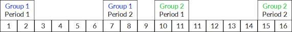
Fig. 1 The ‘stacked’
approach.
In the ‘staggered’ approach we squash the first period of the second group in the washout of the first. Not only faster (which is a nice side effect) but if we apply the \(\small{G\times T}\) test in model \(\small{(\text{I})}\), it’s less likely that something weird will happen than in the ‘stacked’ approach. Furthermore, one gets ammunition in an argument with assessors because the interval between groups is substantially smaller than in the ‘stacked’ approach.
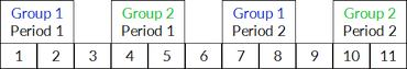
Fig. 2 The ‘staggered’
approach.
Statistics
Hypotheses
The lower and upper limits of the bioequivalence (BE) range \(\small{\{\theta_1,\theta_2\}}\) are defined based on the ‘clinically relevant difference’ \(\small{\Delta}\) assuming log-normal distributed data \[\left\{\theta_1=100\,(1-\Delta),\,\theta_2=100\,(1-\Delta)^{-1}\right\}\tag{1}\] Commonly \(\small{\Delta}\) is set to 0.20. Hence, we obtain: \[\left\{\theta_1=80.00\%,\,\theta_2=125.00\%\right\}\tag{2}\]
Conventionally BE is assessed by the confidence interval (CI) inclusion approach: \[H_0:\frac{\mu_\textrm{T}}{\mu_\textrm{R}}\not\subset\left\{\theta_1,\theta_2\right\}\:vs\:H_1:\theta_1<\frac{\mu_\textrm{T}}{\mu_\textrm{R}}<\theta_2\tag{3}\]
As long as the \(\small{100\,(1-2\,\alpha)}\) CI lies entirely within the BE margins \(\small{\{\theta_1,\theta_2\}}\), the Null Hypothesis \(\small{H_0}\) of inequivalence in \(\small{(3)}\) is rejected and the Alternative Hypothesis \(\small{H_1}\) of equivalence in \(\small{(3)}\) is accepted.
Models
“The totality of data is analyzed with a new term in the analysis of variance (ANOVA), a Treatment × Group interaction term. This is a measure (on a log scale) of how the ratios of test to reference differ in the groups. For example, if the ratios are very much the same in each group, the interaction would be small or negligible. If interaction is large, as tested in the ANOVA, then the groups cannot be combined. However, if at least one of the groups individually passes the confidence interval criteria, then the test product would be acceptable. If interaction is not statistically significant (p > 0.10), then the confidence interval based on the pooled analysis will determine acceptability.
Slightly different by the FDA. Details are outlined further down.
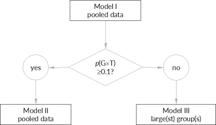
Fig. 3 The
FDA’s decision
scheme.
Models are described in the following ‘bottom to top’. Model \(\small{(\text{III})}\) is the conventional one, i.e., without any group- or site-terms. It can be used for the pooled data or groups / sites separately. Model \(\small{(\text{II})}\) takes the multi-group/-site nature of the study into account, i.e., contains additional / modified terms. Model \(\small{(\text{I})}\) is a pre-test and contains an additional term for the Group-by-Treatment interaction.
Model III (conventional)
The model for a crossover design in average bioequivalence as stated
in guidelines is \[\eqalign{Y&|\;\text{Sequence},\,\text{Subject}(\text{Sequence}),\\
&\phantom{|}\;\text{Period},\,\text{Treatment}\small{\textsf{,}}}{\tag{III}}\]
where \(\small{Y}\) is the response,
i.e. a certain PK metric.
Most regulations recommend an ANOVA,
i.e., all effects are fixed. The
FDA and Health
Canada recommend a mixed-effects
model, i.e., to specify \(\small{\text{Subject}(\text{Sequence})}\)
as a random effect and all others fixed.
It must be mentioned that in comparative bioavailability studies
subjects are usually uniquely coded. Hence, the nested term \(\small{\text{Subject}(\text{Sequence})}\)
in \(\small{(\text{III})}\) is a bogus one9 and could
be replaced by the simple \(\small{\text{Subject}}\) as well. See also
another
article.
Groups and sites were mentioned by the FDA.2
“If a crossover study is carried out in two or more groups of subjects (e.g., if for logistical reasons only a limited number of subjects can be studied at one time), the statistical model should be modified to reflect the multigroup nature of the study. In particular, the model should reflect the fact that the periods for the first group are different from the periods for the second group.
If the study is carried out in two or more groups and those groups are studied at different clinical sites, or at the same site but greatly separated in time (months apart, for example), questions may arise as to whether the results from the several groups should be combined in a single analysis.
Pooling of data is acceptable for Japan’s NIHS under certain conditions.10
“It is acceptable to regard a study in 2 separate groups as a single study, and to analyze the combined data from 2 separate groups, if the following conditions are fulfilled: (1) the study is planned to be conducted in 2 separate groups a priori; (2) the tests are conducted in both groups during the same time period; (3) the same analytical methods are used in both groups; and (4) the number of subjects is similar between the groups.
In the Eurasian Economic Union a modification of the model is mandatory (Article 93), unless a justification is stated in the protocol and discussed with the competent authority (Article 94).4 That’s my interpretation; if you know Russian:
In the EMA’s guideline3 we find only:
“The study should be designed in such a way that the formulation effect can be distinguished from other effects.
The precise model to be used for the analysis should be pre-specified in the protocol. The statistical analysis should take into account sources of variation that can be reasonably assumed to have an effect on the response variable.
A similar wording is given in most other of the global guidelines.
Model II (groups, sites)
If the study is performed in multiple groups or sites, model \(\small{(\text{III})}\) can be modified to \[\eqalign{Y&|\;\text{F},\,\;\text{Sequence},\,\text{Subject}(\text{F}\times \text{Sequence}),\\ &\phantom{|}\;\text{Period}(\text{F}),\;\text{F}\times \text{Sequence},\,\text{Treatment}\small{\textsf{,}}}\tag{II}\] where \(\small{\text{F}}\) is the code for the respective factor or covariate (\(\small{\text{Group}}\) or \(\small{\text{Site}}\)).
Details are given by the FDA in a recently revised draft guidance.5
“Sometimes, groups reflect factors arising from study design and conduct. For example, a PK BE study can be carried out in two or more clinical centers and the study may be considered a multi-group BE study. The combination of multiple factors may complicate the designation of group. Therefore, sponsors should minimize the group effect in a PK BE study as recommended below:Bioequivalence should be determined based on the overall treatment effect in the whole study population. In general, the assessment of BE in the whole study population should be done without including the treatment and group interaction(s) term in the model, but applicants may also use other pre-specified models, as appropriate. The assessment of interaction between the treatment and group(s) is important, especially if any of the first four study design criteria recommended above are not met and the PK BE data are considered pivotal information for drug approval. If the interaction term of group and treatment is significant, heterogeneity of treatment effect across groups should be carefully examined and interpreted with care. If the observed treatment effect of the products varies greatly among the groups, vigorous attempts should be made to find an explanation for the heterogeneity in terms of other features of trial management or subject characteristics, which may suggest appropriate further analysis and interpretation.
- Dose all groups at the same clinic unless multiple clinics are needed to enroll a sufficient number of subjects.
- Recruit subjects from the same enrollment pool to achieve similar demographics among groups.
- Recruit all subjects, and randomly assign them to group and treatment arm, at study outset.
- Follow the same protocol criteria and procedures for all groups.
- When feasible (e.g., when healthy volunteers are enrolled), assign an equal sample size to each group.
[…] the statistical model should reflect the multigroup nature of the study. For example, if subjects are dosed in two groups in a crossover BE study, the model should reflect the fact that the periods for the first group are different from the periods for the second group, i.e., the period effect should be nested within the group effect.
In other words, if the first four conditions are met, assessment of the Group-by-Treatment interaction is considered not important and model \(\small{(\text{II})}\) could be employed.
A similar wording is given in the ICH’s M13A draft guideline.6
“Sample size requirements and/or study logistics may necessitate studies to be conducted with groups of subjects. The BE study should be designed to minimise the group effect in the study. The combination of multiple factors may complicate the designation of group.
BE should be determined based on the overall treatment effect in the whole study population. In general, the assessment of BE in the whole study population should be done without including the Group by Treatment interaction term in the model, but applicants may also use other pre-specified models, as appropriate. However, the appropriateness of the statistical model should be evaluated to account for the multi-group nature of the BE study. Applicants should evaluate potential for heterogeneity of treatment effect across groups, i.e., Group by Treatment interaction. If the Group by Treatment interaction is significant, this should be reported and the root cause of the Group by Treatment interaction should be investigated to the extent possible. Substantial differences in the treatment effect for PK parameters across groups should be evaluated. Further analysis and interpretation may be warranted in case heterogeneity across groups is observed.
In multicentre BE studies, when there are very few subjects in some sites, these subjects may be pooled into one group for consideration in the statistical analysis. Rules for pooling subjects into one group should be pre-specified and a sensitivity analysis is recommended.
Statistical methods and models should be fully pre-specified. Data-driven post hoc analysis is highly discouraged but could be considered only in very rare cases where a very robust scientific justification is provided.
When \(\small{N_\text{F}}\) is the
number of groups or sites, in \(\small{(\text{II})}\) there are \(\small{N_\text{F}-1}\) less residual
degrees of freedom than in \(\small{(\text{III})}\). The table below
gives the designs implemented in PowerTOST.
| design | code | \(\small{t}\) | \(\small{s}\) | \(\small{p}\) | \(\small{f}\) | \(\small{(\text{III})}\) | \(\small{(\text{II})}\) |
|---|---|---|---|---|---|---|---|
| Parallel |
"parallel"
|
\(\small{2}\) | \(\small{-}\) | \(\small{1}\) | \(\small{1}\) | \(\small{\phantom{0}N-2}\) | \(\small{\phantom{0}N-2-(N_\text{F}-1)}\) |
| Paired means |
"paired"
|
\(\small{2}\) | \(\small{-}\) | \(\small{2}\) | \(\small{2}\) | \(\small{\phantom{0}N-1}\) | \(\small{\phantom{0}N-1-(N_\text{F}-1)}\) |
| Crossover |
"2x2x2"
|
\(\small{2}\) | \(\small{2}\) | \(\small{2}\) | \(\tfrac{1}{2}\) | \(\small{\phantom{0}N-2}\) | \(\small{\phantom{0}N-2-(N_\text{F}-1)}\) |
| 2-sequence 3-period full replicate |
"2x2x3"
|
\(\small{2}\) | \(\small{2}\) | \(\small{3}\) | \(\tfrac{3}{8}\) | \(\small{2N-3}\) | \(\small{2N-3-(N_\text{F}-1)}\) |
| 2-sequence 4-period full replicate |
"2x2x4"
|
\(\small{2}\) | \(\small{2}\) | \(\small{4}\) | \(\tfrac{1}{4}\) | \(\small{3N-4}\) | \(\small{3N-4-(N_\text{F}-1)}\) |
| 4-sequence 4-period full replicate |
"2x4x4"
|
\(\small{2}\) | \(\small{4}\) | \(\small{4}\) | \(\tfrac{1}{16}\) | \(\small{3N-4}\) | \(\small{3N-4-(N_\text{F}-1)}\) |
| Partial replicate |
"2x3x3"
|
\(\small{2}\) | \(\small{3}\) | \(\small{3}\) | \(\tfrac{1}{6}\) | \(\small{2N-3}\) | \(\small{2N-3-(N_\text{F}-1)}\) |
| Balaam’s |
"2x4x2"
|
\(\small{2}\) | \(\small{4}\) | \(\small{2}\) | \(\tfrac{1}{2}\) | \(\small{\phantom{0}N-2}\) | \(\small{\phantom{0}N-2-(N_\text{F}-1)}\) |
| Latin Squares |
"3x3"
|
\(\small{3}\) | \(\small{3}\) | \(\small{3}\) | \(\tfrac{2}{9}\) | \(\small{2N-4}\) | \(\small{2N-4-(N_\text{F}-1)}\) |
| Williams’ |
"3x6x3"
|
\(\small{3}\) | \(\small{6}\) | \(\small{3}\) | \(\tfrac{1}{18}\) | \(\small{2N-4}\) | \(\small{2N-4-(N_\text{F}-1)}\) |
| Latin Squares or Williams’ |
"4x4"
|
\(\small{4}\) | \(\small{4}\) | \(\small{4}\) | \(\tfrac{1}{8}\) | \(\small{3N-6}\) | \(\small{3N-6-(N_\text{F}-1)}\) |
code is the design-argument in the
functions of PowerTOST. \(\small{t}\), \(\small{s}\), and \(\small{p}\) are the number of treatments,
sequences, and periods, respectively. \(\small{f}\) is the factor in the radix of
\(\small{(4)}\)
and \(\small{N}\) is the total number
of subjects, i.e., \(\small{N=\sum_{i=1}^{i=s}n_i}\).
The back-transformed \(\small{1-2\,\alpha}\) Confidence Interval (CI) is calculated by \[\text{CI}=100\,\exp\left(\overline{\log_{e}x_\text{T}}-\overline{\log_{e}x_\text{R}}\mp t_{df,\alpha}\sqrt{f \times\widehat{s^2}\sum_{i=1}^{i=s}\frac{1}{n_i}}\,\right)\small{\textsf{,}}\tag{4}\] where \(\small{\overline{\log_{e}x_\text{T}}}\) and \(\small{\overline{\log_{e}x_\text{R}}}\) are the arithmetic11 means of the \(\small{\log_{e}}\)-transformed responses of the test and reference treatments, \(\widehat{s^2}\) is the estimated (residual) variance of the model, and \(\small{n_i}\) is the number of subjects in the \(\small{i^\text{th}}\) of \(\small{s}\) sequences.
Therefore, the CI by \(\small{(4)}\) for given \(\small{N}\) and \(\small{\widehat{s^2}}\) by \(\small{(\text{II})}\) will be consistently wider (more conservative) than that by \(\small{(\text{III})}\) due to the \(\small{N_\text{F}-1}\) fewer degrees of freedom and hence, larger \(\small{t}\)-value. Note that \(\small{\widehat{s^2}}\) is generally slightly different in both models whereas the Point Estimates (PEs) identical. Unless the sample size is small and the number of groups or sites large, the difference in \(\small{\widehat{s^2}}\) and degrees of freedom and hence, the power of the study, is generally negligible.
Let us explore an example: CV 0.30, T/R-ratio 0.95, targeted at 80% power, two groups of 20 subjects each.
sim.BE <- function(CV, theta0 = 0.95, theta1 = 0.80, theta2 = 1.25,
                   target = 0.80, groups = 2, capacity, split = c(0.5, 0.5),
                   mue =  c(0.95, 1 / 0.95), setseed = TRUE, nsims = 1e4,
                   progr = FALSE) {
  require(PowerTOST)
  #######################
  # Generate study data #
  #######################
  group.data <- function(CV = CV, mue = mue, n.group = n.group,
                         capacity = capacity) {
    if (length(n.group) < 2) stop("At least two groups required.")
    if (length(mue) == 1) mue <- c(mue, 1 / mue)
    if (max(n.group) > capacity)
      warning("Largest group exceeds capacity of site!")
    subject <- rep(1:sum(n.group), each = 2)
    group   <- period <- treatment <- sequence <- NULL
    for (i in seq_along(n.group)) {
      sequence  <- c(sequence, c(rep("TR", n.group[i]),
                               c(rep("RT", n.group[i]))))
      treatment <- c(treatment, rep(c("T", "R"), ceiling(n.group[i] / 2)),
                                rep(c("R", "T"), floor(n.group[i] / 2)))
      period    <- c(period, rep(c(1:2), ceiling(n.group[i] / 2)),
                             rep(c(1:2), floor(n.group[i] / 2)))
      group     <- c(group, rep(i, ceiling(n.group[i])),
                            rep(i, floor(n.group[i])))
    }
    data        <- data.frame(subject, group, sequence, treatment, period,
                              Y = NA_real_)
    for (i in seq_along(n.group)) {
      if (length(CV) == 1) { # homogenicity
        data$Y[data$group == i & data$treatment == "T"] <-
          exp(mue[i] + rnorm(n = n.group[i], mean = 0, sd = CV2se(CV)))
        data$Y[data$group == i & data$treatment == "R"] <-
          exp(1 + rnorm(n = n.group[i], mean = 0, sd = CV2se(CV)))
      } else {                # heterogenicity
        data$Y[data$group == i & data$treatment == "T"] <-
          exp(mue[i] + rnorm(n = n.group[i], mean = 0, sd = CV2se(CV[1])))
        data$Y[data$group == i & data$treatment == "R"] <-
          exp(1 + rnorm(n = n.group[i], mean = 0, sd = CV2se(CV[2])))
      }
    }
    facs   <- c("subject", "group", "sequence", "treatment", "period")
    data[facs] <- lapply(data[facs], factor)
    return(data)
  }
  ########################
  # Initial computations #
  ########################
  if (length(CV) == 1) {
    CVp <- CV
  } else {
    if (length(CV) == 2) {
      CVp <- mse2CV(mean(c(CV2mse(CV[1]), CV2mse(CV[2]))))
   } else {
      stop ("More than two CVs not supported.")
    }
  }
  n       <- sampleN.TOST(CV = CVp, theta0 = theta0, theta1 = theta1,
                          theta2 = theta2, design = "2x2x2",
                          targetpower = target, print = FALSE)[["Sample size"]]
  n.group <- as.integer(n * split)
  if (sum(n.group) < n) {  # increase size of last group if necessary
    n.group[groups] <- n.group[groups] + n - sum(n.group)
    }
  III     <- II <- data.frame(MSE = rep(NA_real_, nsims), CV = NA_real_,
                              PE = NA_real_, lower = NA_real_, upper = NA_real_,
                              BE = FALSE, power = NA_real_)
  if (setseed) set.seed(123456)
  if (progr) pb <- txtProgressBar(style = 3)
  ###############
  # Simulations #
  ###############
  ow      <- options()
  options(contrasts = c("contr.treatment", "contr.poly"), digits = 12)
  for (sim in 1:nsims) {
    data          <- group.data(CV = CV, mue = mue, n.group = n.group,
                                capacity = capacity)
    model.III     <- lm(log(Y) ~ sequence +
                                 treatment +
                                 subject %in% sequence +
                                 period, data = data)
    III$MSE[sim]  <- anova(model.III)["Residuals", "Mean Sq"]
    III$CV[sim]   <- mse2CV(III$MSE[sim])
    III$PE[sim]   <- 100 * exp(coef(model.III)[["treatmentT"]])
    III[sim, 4:5] <- 100 * exp(confint(model.III, "treatmentT",
                                       level = 0.9))
    if (round(III$lower[sim], 2) >= 100 * theta1 &
        round(III$upper[sim], 2) <= 100 * theta2) III$BE[sim] <- TRUE
    III$power[sim] <- power.TOST(CV = mse2CV(III$MSE[sim]),
                                 theta0 = III$PE[sim] / 100, n = n)
    model.II      <- lm(log(Y) ~ group +
                                 sequence +
                                 treatment +
                                 subject %in% (group * sequence) +
                                 period %in% group +
                                 group:sequence, data = data)
    II$MSE[sim]   <- anova(model.II)["Residuals", "Mean Sq"]
    II$CV[sim]    <- mse2CV(II$MSE[sim])
    II$PE[sim]    <- 100 * exp(coef(model.II)[["treatmentT"]])
    II[sim, 4:5]  <- 100 * exp(confint(model.II, "treatmentT",
                                       level = 0.9))
    if (round(II$lower[sim], 2) >= 100 * theta1 &
        round(II$upper[sim], 2) <= 100 * theta2) II$BE[sim] <- TRUE
    II$power[sim] <- power.TOST(CV = mse2CV(II$MSE[sim]),
                                theta0 = II$PE[sim] / 100, n = n)
    if (progr) setTxtProgressBar(pb, sim / nsims)
  }
  options(ow)
  if (progr) close(pb)
  return(list(III = III, II = II))
}
CV     <- 0.30
theta0 <- 0.95
target <- 0.80
nsims  <- 1e5
x      <- sampleN.TOST(CV = CV, theta0 = theta0, targetpower = target,
                       print = FALSE)
y      <- sim.BE(CV = CV, theta0 = 0.95, target = 0.80,
                 capacity = 20, mue = c(0.95, 1/0.95), nsims = nsims)
MSE    <- data.frame(Model  = c("III", "II"),
                     median = c(sprintf("%.6f", median(y$III$MSE)),
                                sprintf("%.6f", median(y$II$MSE))),
                     min = c(sprintf("%.6f", min(y$III$MSE)),
                             sprintf("%.6f", min(y$II$MSE))),
                     max = c(sprintf("%.6f", max(y$III$MSE)),
                             sprintf("%.6f", max(y$II$MSE))),
                     df  = c(x[["Sample size"]] - 2, x[["Sample size"]] - 3))
power  <- data.frame(Model = c("III", "II"),
                     median = c(sprintf("%.4f", median(y$III$power)),
                                sprintf("%.4f", median(y$II$power))),
                     min = c(sprintf("%.4f", min(y$III$power)),
                             sprintf("%.4f", min(y$II$power))),
                     max = c(sprintf("%.4f", max(y$III$power)),
                             sprintf("%.4f", max(y$II$power))))
cat(formatC(nsims, format = "d", big.mark = ","), "simulations")
cat("\n Comparison of residual mean squares error",
    sprintf("(expected for Model III %.6f)\n", CV2mse(CV)))
print(MSE, row.names = FALSE, right = FALSE)
cat(" Comparison of power",
    sprintf("(expected for Model III %.4f)\n", x[["Achieved power"]]))
print(power, row.names = FALSE, right = FALSE)
cat("Are all Point Estimates equal?\n")
all.equal(y$III$PE, y$II$PE)
# 100,000 simulations
# Comparison of residual mean squares error (expected for Model III 0.086178)
# Model median min max df
# III 0.085943 0.028431 0.199054 38
# II 0.085891 0.029144 0.203947 37
# Comparison of power (expected for Model III 0.8158)
# Model median min max
# III 0.8138 0.0036 0.9998
# II 0.8135 0.0035 0.9999
# Are all Point Estimates equal?
# [1] TRUEAs expected, \(\small{\widehat{s^2}}\) is similar and the PEs obtained by both models are identical – if sequences are balanced and group sizes identical, but different in the case of imbalanced sequences and unequal group sizes.
In a 2×2×2 crossover design the residual degrees of freedom for \(\small{(4)}\) in the models are \[\eqalign{(\text{III}):df&=N-2\\ (\text{II}):df&=N-2-(N_\text{F}-1)\small{\textsf{,}}}\tag{5}\] where \(\small{N}\) is total number of subjects and \(\small{N_\text{F}}\) the number of groups or sites.
Let us continue the example. This time two to eight groups (or sites).
CV  <- 0.30
MSE <- CV2mse(CV)
n   <- sampleN.TOST(CV = CV, theta0 = 0.95, targetpower = 0.80,
                    print = FALSE)[["Sample size"]]
n1  <- n2 <- n / 2
NF  <- c(2:4, 6, 8)
x   <- data.frame(n = n, NF = NF,
                  df.3 = n - 2,
                  CL.lo.3 = NA_real_, CL.hi.3 = NA_real_,
                  width.3 = NA_real_,
                  df.2 = n - 2 - (NF - 1),
                  CL.lo.2 = NA_real_, CL.hi.2 = NA_real_,
                  width.2 = NA_real_)
for (i in seq_along(NF)) {
  x[i, 4:5] <- exp(log(theta0) - log(1) + c(-1, +1) *
                   qt(1 - 0.05, df = x$df.3[i]) *
                   sqrt(MSE / 2 * (1 / n1 + 1 / n2)))
  x[i, 8:9] <- exp(log(theta0) - log(1) + c(-1, +1) *
                   qt(1 - 0.05, df = x$df.2[i]) *
                   sqrt(MSE / 2 * (1 / n1 + 1 / n2)))
}
x$width.3 <- x$CL.hi.3 - x$CL.lo.3
x$width.2 <- x$CL.hi.2 - x$CL.lo.2
diffs     <- x$width.2 - x$width.3
names(x)[c(1, 3:5, 7:9)] <- c("N", "df (III)", "CL.lo (III)", "CL.hi (III)",
                              "df (II)", "CL.lo (II)", "CL.hi (II)")
x[, 4] <- sprintf("%.2f%%", 100 * x[, 4])
x[, 5] <- sprintf("%.2f%%", 100 * x[, 5])
x[, 8] <- sprintf("%.2f%%", 100 * x[, 8])
x[, 9] <- sprintf("%.2f%%", 100 * x[, 9])
print(x[, c(1:5, 7:9)], row.names = FALSE)
cat("Maximum difference in the width of CIs:",
    sprintf("%.2g%%.\n", 100 * max(diffs)))
# N NF df (III) CL.lo (III) CL.hi (III) df (II) CL.lo (II) CL.hi (II)
# 40 2 38 85.05% 106.12% 37 85.04% 106.13%
# 40 3 38 85.05% 106.12% 36 85.03% 106.13%
# 40 4 38 85.05% 106.12% 35 85.03% 106.14%
# 40 6 38 85.05% 106.12% 33 85.01% 106.16%
# 40 8 38 85.05% 106.12% 31 84.99% 106.18%
# Maximum difference in the width of CIs: 0.12%.As stated above, the difference in the widths of CIs is negligible in any case. If we have just two groups or sites the difference in the width of CIs is <0.01%.
Model I
No details are given (see the quote above) by the FDA how the Group-by-Treatment interaction should be tested.5 However, this text can be found under the FOI12 and in deficiency letters:
The following statistical model can be applied: \[\eqalign{Y&|\;\text{Group},\,\text{Sequence},\,\text{Treatment},\\ &\phantom{|}\;\text{Subject}(\text{Group}\times \text{Sequence}),\,\text{Period}(\text{Group}),\\ &\phantom{|}\;\text{Group}\times \text{Sequence},\,\text{Group}\times \text{Treatment}\small{\textsf{,}}}\tag{I}\] where \(\small{\text{Subject}(\text{Group}\times \text{Sequence})}\) is a random effect and all other effects are fixed effects.
- If the Group-by-Treatment interaction test is not statistically significant (p ≥0.1), only the Group-by-Treatment term can be dropped from the model. → (II)
- If the Group-by-Treatment interaction is statistically significant (p <0.1), DBE requests that equivalence be demonstrated in one of the groups, provided that the group meets minimum requirements for a complete BE study. → (III)
- […] the statistical analysis for BE studies dosed in more than one group should commence only after all subjects have been dosed and all pharmacokinetic parameters have been calculated. Statistical analysis to determine BE within each dosing group should never be initiated prior to dosing the next group […].
- If ALL of the following criteria are met, it may not be
necessary to include Group-by-Treatment in the statistical model:
- the clinical study takes place at one site;
- all study subjects have been recruited from the same enrollment pool;
- all of the subjects have similar demographics;
- all enrolled subjects are randomly assigned to treatment groups at study outset.
- In this latter case, the appropriate statistical model would include
only the factors
Sequence, Period, Treatment and Subject (nested within Sequence). → (III)
It must be mentioned that due to the \(\small{\text{Group}\times \text{Treatment}}\) term in this model the treatment effect is biased and hence, must not be used to assess BE.
Contrary to what was stated in these deficiency letters, if the four criteria are met, model \(\small{(\text{II})}\) – instead of model \(\small{(\text{III})}\) – could be employed.5 If at least one of these criteria is not met and the interaction term of group and treatment in model \(\small{(\text{I})}\) is significant,
“[…] heterogeneity of treatment effect across groups should be carefully examined and interpreted with care. If the observed treatment effect of the products varies greatly among the groups, vigorous attempts should be made to find an explanation for the heterogeneity in terms of other features of trial management or subject characteristics, which may suggest appropriate further analysis and interpretation.
Regrettably the WHO stated also:13
“In those cases where the subjects are recruited and treated in groups, it is appropriate to investigate the statistical significance of the group-by-formulation interaction e.g., with the following ANOVA model: Group, Sequence, Formulation, Period (nested within Group), Group-by-Sequence interaction, Subject (nested within Group*Sequence) and Group-by-Formulation interaction. If this interaction is significant, the study results are not interpretable. However, it is not considered to be correct to report the results of the 90% confidence interval of the ratio test/comparator based on the standard error derived from this ANOVA. If the group-by-formulation interaction is not significant, the 90% confidence interval should be calculated based on the ANOVA model defined in the protocol. This model may or may not include the group effect as pre-defined in the protocol. This depends on whether the group effect is believed to explain the variability observed in the data.
On the contrary, my dear Dr. Watson! It is not
appropriate.
At least we can state in the protocol that we don’t believe
[sic] in a group-by-treatment interaction. Believes14 don’t
belong to the realm of science – only assumptions do.
Power
The function power.TOST.sds() of PowerTOST
supports simulations of models \(\small{\text{(I)}}\), \(\small{\text{(II)}}\) and \(\small{\text{(III)}}\) of studies in a
2×2×2 crossover, as well as in full (except Balaam’s) and partial
replicate designs.
The script supports sample size estimation for average bioequivalence
and generation of groups based on the clinical capacity, where sequences
within groups will be balanced.
The estimated sample size can be adjusted based on an anticipated
dropout-rate. If this is selected, i.e.,
do.rate > 0, two simulations are performed:
- One for the adjusted sample size (no dropouts, optimistic) and
Realization: Observations (in a sample) of a random variable (of the population).
- one for the estimated sample size (dropout-rate realized, pessimistic).
Two options for the generation of groups are supported by the logical
argument equal:
FALSE: Attempts to generate at least one group with the maximum size of the clinical site (default).TRUE: Attempts to generate equally sized groups.
Finally, power by \(\small{\text{(II)}}\) or – if
gmodel = 1 the
FDA’s decision scheme – is compared to exact power by \(\small{\text{(III)}}\).
As we have seen in the table above, due to its
lower degrees of freedom power of \(\small{\text{(II)}}\) should always be
lower than the one of \(\small{\text{(III)}}\). If you get a
positive change value in the comparison, it is a simulation
artifact. In such a case, increase the number of simulations
(nsims = 1e6 or higher). Cave: 182
LOC.
sim.groups <- function(CV, theta0 = 0.95, theta1, theta2, target = 0.80,
                       design = "2x2x2", capacity, equal = FALSE,
                       gmodel = 2, do.rate = 0, nsims = 1e5L, show = TRUE) {
  ##########################################################
  # Explore the impact on power of a group model com-      #
  # pared to the conventional model of pooled data via     #
  # simulations.                                           #
  # ------------------------------------------------------ #
  # capacity: maximum capacity of the clinical site        #
  # equal:    TRUE : tries to generate equally sized       #
  #                  groups                                #
  #           FALSE: tries to get at least one group with  #
  #                  the maximum size of the clinical site #
  #                  (default)                             #
  # do.rate:  anticipated dropout-rate; if > 0 a second    #
  #           simulation is performed based on the adjust- #
  #           ed sample size                               #
  ##########################################################
  if (missing(theta1) & missing(theta2)) theta1 <- 0.80
  if (missing(theta1)) theta1 <- 1 / theta2
  if (missing(theta2)) theta2 <- 1 / theta1
  if (theta0 < theta1 | theta0 > theta2)
    stop("theta0 must be within {theta1, theta2}.", call. = FALSE)
  if (theta0 == theta1 | theta0 == theta2)
    stop("Simulation of the Type I Error not supported.",
         "\n       Use power.TOST.sds() directly.", call. = FALSE)
  if (!design %in% c("2x2", "2x2x2", "2x3x3", "2x2x4", "2x2x3"))
    stop("Design \"", design, "\" not implemented.", call. = FALSE)
  ns <- as.integer(substr(design, 3, 3))
  make.equal <- function(n, ns) {
    # make equally sized sequences
    return(as.integer(ns * (n %/% ns + as.logical(n %% ns))))
  }
  nadj <- function(n, do.rate, ns) {
    # adjust the sample size
    return(as.integer(make.equal(n / (1 - do.rate), ns)))
  }
  grouping <- function(capacity, n, design, equal, do.rate) {
    # based on the sample size and capacity, calculate the
    # number of groups and subjects / group
    if (do.rate == 0) {
      x <- n
      stop.txt <- paste("The sample size of", x)
    } else {
      x <-  nadj(n, do.rate, ns)
      stop.txt <- paste("The adjusted sample size of", x)
    }
    if (x <= capacity) {
        stop(stop.txt, " does not exhaust the clinical capacity.",
             call. = FALSE)
    } else {
    # split sample size into >=2 groups based on capacity
    # TODO: Handle a case where with no dropouts <= capacity (no grouping)
    #       but with the adjusted sample size two groups are required
      if (equal) { # attempt to make all groups equally sized
        grps <- ceiling(n / capacity)
        tmp  <- rep(n / grps, grps)
        ngrp <- make.equal(tmp, ns)
        if (!isTRUE(all.equal(tmp, ngrp)))
          message("Note: Imbalanced sequences in groups (",
                  paste(round(tmp, 0), collapse = "|"), ") corrected.\n")
        if (sum(ngrp) > n) ngrp[length(ngrp)] <- n-sum(ngrp[-1])
      } else {     # at least one group = capacity
        ngrp    <- rep(0, ceiling(n / capacity))
        grps    <- length(ngrp)
        ngrp[1] <- capacity
        for (j in 2:grps) {
          n.tot <- sum(ngrp) # what we have so far
          if (n.tot + capacity <= n) {
            ngrp[j] <- capacity
        } else {
            ngrp[j] <- n - n.tot
          }
        }
      }
    }
    return(ngrp = list(grps = length(ngrp), ngrp = ngrp))
  }
  if (equal) {
    txt <- "Attempting to generate equally sized groups."
} else {
    txt <- paste("Attempting to have at least one group with",
                 "\nthe maximum capacity of the clinical site.")
  }
  txt    <- paste(txt, "\nCV                   :", sprintf("%.4f", CV),
                  "\ntheta0               :", sprintf("%.4f", theta0),
                  "\nBE-limits            :",
                  sprintf("%.4f – %.4f", theta1, theta2),
                  "\nTarget power         :", sprintf("%.2f", target),
                  "\nDesign               :", design,
                  "\nClinical capacity    :", capacity)
  tmp    <- sampleN.TOST(CV = CV, theta0 = theta0, theta1 = theta1,
                         theta2 = theta2, targetpower = target,
                         design = design, print = FALSE)
  res    <- data.frame(n = NA_integer_, grps = NA_integer_,
                       n.grp = NA_integer_, m.1 = NA_real_, m.2 = NA_real_,
                       change = NA_real_)
  res$n  <- tmp[["Sample size"]]
  res[4] <- tmp[["Achieved power"]]
  x      <- grouping(capacity, res$n, design, equal, do.rate)
  res[2] <- x[["grps"]]
  ngrp   <- x[["ngrp"]]
  res[3] <- paste(ngrp, collapse = " | ")
  res[5] <- power.TOST.sds(CV = CV, theta0 = theta0, theta1 = theta1,
                           theta2 = theta2, n = res$n,
                           design = design, grps = res$grps, ngrp = ngrp,
                           gmodel = gmodel, progress = FALSE, nsims = nsims)
  res[6] <- 100 * (res$m.2 - res$m.1) / res$m.1
  des    <- known.designs()[2:3]
  df     <- as.expression(des$df[des$design == design])
  dfs    <- rep(NA_integer_, 2)
  n      <- res$n
  dfs[1] <- as.integer(eval(parse(text = df)))
  dfs[2] <- as.integer(dfs[1] - (res$grps - 1))
  txt    <- paste(txt, paste0("\n", paste(rep("—", 46), collapse = "")),
                  "\nTotal sample size    :", res$n,
                  "\nNumber of groups     :", sprintf("%2.0f", res[2]),
                  "\nSubjects per group   :", res[3],
                  "\nDegrees of freedom   :",
                  sprintf("%3i", dfs[1]), "(model III)",
                  "\n                      ",
                  sprintf("%3i", dfs[2]), "(model II)")
  if (do.rate > 0) {
    res[2, 1] <- nadj(n, do.rate, ns)
    res[2, 4] <- signif(power.TOST(CV = CV, theta0 = theta0, theta1 = theta1,
                                   theta2 = theta2, n = res$n[2],
                                   design = design), 4)
    x         <- grouping(capacity, res$n[2], design, equal, do.rate)
    res[2, 2] <- x[["grps"]]
    ngrp      <- x[["ngrp"]]
    res[2, 3] <- paste(ngrp, collapse = " | ")
    res[2, 5] <- power.TOST.sds(CV = CV, theta0 = theta0, theta1 = theta1,
                                theta2 = theta2, n = res$n[2],
                                design = design, grps = res$grps, ngrp = ngrp,
                                gmodel = gmodel, progress = FALSE, nsims = nsims)
    res[2, 6] <- 100 * (res$m.2[2] - res$m.1[2]) / res$m.1[2]
    dfs       <- rep(NA_integer_, 2)
    n         <- res$n[2]
    dfs[1]    <- as.integer(eval(parse(text = df)))
    dfs[2]    <- as.integer(dfs[1] - (res$grps[2] - 1))
    txt    <- paste(txt, paste0("\n", paste(rep("—", 46), collapse = "")),
                    "\nAnticip. dropout-rate:",
                    sprintf("%2g%%", 100 * do.rate),
                    "\nAdjusted sample size :", res$n[2],
                    "\nNumber of groups     :", sprintf("%2.0f", res[2, 2]),
                    "\nSubjects per group   :", res[2, 3],
                    "\nDegrees of freedom   :",
                    sprintf("%3i", dfs[1]), "(model III)",
                    "\n                      ",
                    sprintf("%3i", dfs[2]), "(model II)")
  }
  res[, 4] <- sprintf("%6.4f", res[, 4])
  res[, 5] <- sprintf("%6.4f", res[, 5])
  res[, 6] <- sprintf("%+.3f%%", res[, 6])
  names(res)[4:6] <- c("model III", "model II", "change")
  names(res)[c(4, 6)] <- c("model III", "change")
  if (gmodel == 1) {
    names(res)[5] <- "decision scheme"
 } else {
    names(res)[5] <- "model II"
  }
  txt    <- paste0(txt, paste0("\n", paste(rep("—", 46), collapse = "")),
                   "\nAchieved power of model III and ")
  if (gmodel == 1) {
    txt <- paste0(txt, "the decision scheme;",
                  "\nrelative change in power of the decision scheme",
                  "\ncompared to model III:\n\n")

 } else {
    txt <- paste0(txt, "II;",
                  "\nrelative change in power of model II",
                  "\ncompared to model III:\n\n")
  }
  if (show) cat(txt)
  if (do.rate == 0) {
    print(res[, c(1, 4:6)], row.names = FALSE)
 } else {
    row.names(res) <- c("Expected", "Adjusted")
    print(res[, c(1, 4:6)])
  }
  return(result = list(power = res, df = dfs))
}
Say, the assumed CV is 31%, the T/R-ratio 0.95, and we plan the study for ≥ 80% power in a 2×2×2 crossover design. The capacity of the clinical site is 24. We anticipate a dropout-rate of 5% and adjust the sample size accordingly (i.e., dose more subjects in order to have at least as many eligible subjects than estimated for the target power). We want to have at least one group with the capacity of the site.
CV       <- 0.31
theta0   <- 0.95
target   <- 0.80
design   <- "2x2x2"
capacity <- 24
do.rate  <- 0.05
x <- sim.groups(CV = CV, theta0 = theta0, target = target,
                design = design, capacity = capacity, do.rate = do.rate)
# Attempting to have at least one group with
# the maximum capacity of the clinical site.
# CV : 0.3100
# theta0 : 0.9500
# BE-limits : 0.8000 – 1.2500
# Target power : 0.80
# Design : 2x2x2
# Clinical capacity : 24
# ——————————————————————————————————————————————
# Total sample size : 42
# Number of groups : 2
# Subjects per group : 24 | 18
# Degrees of freedom : 40 (model III)
# 39 (model II)
# ——————————————————————————————————————————————
# Anticip. dropout-rate: 5%
# Adjusted sample size : 46
# Number of groups : 2
# Subjects per group : 24 | 22
# Degrees of freedom : 44 (model III)
# 43 (model II)
# ——————————————————————————————————————————————
# Achieved power of model III and II;
# relative change in power of model II
# compared to model III:
#
# n model III model II change
# Expected 42 0.8113 0.8107 -0.072%
# Adjusted 46 0.8451 0.8428 -0.276%In \(\small{\text{(II)}}\) we loose only one degree of freedom compared to \(\small{\text{(III)}}\). Hence, the loss in power is negligible.
For Japan’s
NIHS model \(\small{\text{(III)}}\) is acceptable if
groups are of similar sizes.10 Hence, we
specify equal = TRUE.
CV       <- 0.31
theta0   <- 0.95
target   <- 0.80
design   <- "2x2x2"
capacity <- 24
do.rate  <- 0.05
x <- sim.groups(CV = CV, theta0 = theta0, target = target,
                design = design, capacity = capacity, equal = TRUE,
                do.rate = do.rate)
# Note: Imbalanced sequences in groups (21|21) corrected.# Note: Imbalanced sequences in groups (23|23) corrected.# Attempting to generate equally sized groups.
# CV : 0.3100
# theta0 : 0.9500
# BE-limits : 0.8000 – 1.2500
# Target power : 0.80
# Design : 2x2x2
# Clinical capacity : 24
# ——————————————————————————————————————————————
# Total sample size : 42
# Number of groups : 2
# Subjects per group : 22 | 20
# Degrees of freedom : 40 (model III)
# 39 (model II)
# ——————————————————————————————————————————————
# Anticip. dropout-rate: 5%
# Adjusted sample size : 46
# Number of groups : 2
# Subjects per group : 24 | 22
# Degrees of freedom : 44 (model III)
# 43 (model II)
# ——————————————————————————————————————————————
# Achieved power of model III and II;
# relative change in power of model II
# compared to model III:
#
# n model III model II change
# Expected 42 0.8113 0.8108 -0.062%
# Adjusted 46 0.8451 0.8428 -0.276%We are notified that equal group sizes (21|21 and 23|23) would not be balanced. However, the resulting group sizes are similar (22|20 and 24|22). If the other conditions are fullfilled, we may use model \(\small{\text{(III)}}\).
Another example demonstrating that we don’t have to worry about loss in power and can readily employ the common sample size estimation. An HVD (assumed CV 30 – 40%, conservative T/R-ratio 0.90), one to six sites, study planned for ≥ 80% power in a 2-sequence 4-period full replicate design.
CV     <- seq(0.3, 0.40, 0.05)
theta0 <- 0.90
sites  <- 1:6L
target <- 0.80
design <- "2x2x4"
supps  <- known.designs()[c(2:3, 10, 8, 7), 2:3]
if (!design %in% supps$design)
  stop("Group model for \"", design, "\" design not supported.")
n.est  <- numeric(length(CV))
for (i in seq_along(CV)) {# conventional sample size
  n.est[i] <- sampleN.TOST(CV = CV[i], theta0 = theta0,
                           targetpower = target, design = design,
                           print = FALSE)[["Sample size"]]
}
res    <- data.frame(CV = rep(CV, each = length(sites)),
                     n = rep(n.est, each = length(sites)),
                     df.III = NA_real_,
                     power.III = NA_real_, sites = sites,
                     df.II = NA_real_,
                     power.II = NA_real_)
# power by subject data simulations (sds)
# extremely slow with one million simulations
for (i in 1:nrow(res)) {
  n  <- res$n[i]
  df <- as.expression(supps$df[supps$design == design])
  if (res$sites[i] == 1) {# power of model III
    res$df.III[i]    <- as.integer(eval(parse(text = df)))
    res$power.III[i] <- power.TOST.sds(CV = res$CV[i],
                                       theta0 = theta0,
                                       n = res$n[i],
                                       grps = res$sites[i],
                                       design = design,
                                       gmodel = 3, nsims = 1e6,
                                       progress = FALSE)
}else {                # power of model II
    res$df.II[i]     <- as.integer(eval(parse(text = df)) - (res$sites[i] - 1))
    res$power.II[i]  <- power.TOST.sds(CV = res$CV[i],
                                       theta0 = theta0,
                                       n = res$n[i],
                                       grps = res$sites[i],
                                       design = design,
                                       gmodel = 2, nsims = 1e6,
                                       progress = FALSE)
  }
}
# cosmetics
res$df.III[is.na(res$df.III)] <- "- "
res$df.II[is.na(res$df.II)]   <- "- "
names(res)[c(3, 6)]           <- "df"
res$power.III <- sprintf("%.5f", res$power.III)
res$power.II  <- sprintf("%.5f", res$power.II)
res$power.III[which(res$power.III == "NA")] <- "-     "
res$power.II[which(res$power.II == "NA")]   <- "-     "
print(res, row.names = FALSE)
# CV n df power.III sites df power.II
# 0.30 40 116 0.81002 1 - -
# 0.30 40 - - 2 115 0.81003
# 0.30 40 - - 3 114 0.80866
# 0.30 40 - - 4 113 0.80982
# 0.30 40 - - 5 112 0.80962
# 0.30 40 - - 6 111 0.80442
# 0.35 52 152 0.80043 1 - -
# 0.35 52 - - 2 151 0.80039
# 0.35 52 - - 3 150 0.79934
# 0.35 52 - - 4 149 0.79829
# 0.35 52 - - 5 148 0.79910
# 0.35 52 - - 6 147 0.79708
# 0.40 68 200 0.80739 1 - -
# 0.40 68 - - 2 199 0.80735
# 0.40 68 - - 3 198 0.80681
# 0.40 68 - - 4 197 0.80612
# 0.40 68 - - 5 196 0.80642
# 0.40 68 - - 6 195 0.80524See a rather strange example, where an agency required \(\small{\text{(III)}}\) – separate for groups – because one of six \(\small{G\times T}\) tests (three PK metrics of two APIs of an FDC) was significant.
CV     <- 0.32
theta0 <- 0.95
target <- 0.90
design <- "2x2x2"
x      <- sampleN.TOST(CV = CV, theta0 = theta0, targetpower = target,
                  design = design, print = FALSE)
n      <- x[["Sample size"]]
power  <- x[["Achieved power"]]
x      <- data.frame(groups = 1:3, n.group = n / 1:3,
                     power.group = c(power, rep(NA_real_, 2)))
for (i in 2:3) {
  x$power.group[i] <- suppressMessages(
                        power.TOST(CV = CV, theta0 = theta0,
                                   n = x$n.group[i],
                                   design = design))
}
names(x)[2:3] <- c("n/group", "power/group")
print(x, row.names = FALSE)
# groups n/group power/group
# 1 60 0.9080189
# 2 30 0.6212292
# 3 20 0.3626223There were only two groups and the company was lucky because T/R-ratios and CVs were ‘better’ than assumed, as well as the dropout-rate lower than anticipated in the sample size estimation. Impossible that all would have passed if there would have been three groups (power < 50% is always a failure).
Let’s assume you are a victim of an agency requiring the FDA’s decision scheme (\(\small{\text{I}}\) → \(\small{\text{II}}\) or \(\small{\text{III}}\)).
# Cave: extremely long runtime
CV       <- 0.31
theta0   <- 0.95
target   <- 0.80
design   <- "2x2x2"
capacity <- 24
do.rate  <- 0.05
x <- sim.groups(CV = CV, theta0 = theta0, target = target,
                design = design, capacity = capacity, do.rate = do.rate,
                gmodel = 1)
# Attempting to have at least one group with
# the maximum capacity of the clinical site.
# CV : 0.3100
# theta0 : 0.9500
# BE-limits : 0.8000 – 1.2500
# Target power : 0.80
# Design : 2x2x2
# Clinical capacity : 24
# ——————————————————————————————————————————————
# Total sample size : 42
# Number of groups : 2
# Subjects per group : 24 | 18
# Degrees of freedom : 40 (model III)
# 39 (model II)
# ——————————————————————————————————————————————
# Anticip. dropout-rate: 5%
# Adjusted sample size : 46
# Number of groups : 2
# Subjects per group : 24 | 22
# Degrees of freedom : 44 (model III)
# 43 (model II)
# ——————————————————————————————————————————————
# Achieved power of model III and the decision scheme;
# relative change in power of the decision scheme
# compared to model III:
#
# n model III decision scheme change
# Expected 42 0.8113 0.7653 -5.674%
# Adjusted 46 0.8451 0.7924 -6.232%Note that we simulated no Group-by-Treatment interaction! Nevertheless, in 10% of cases the \(\small{G\times T}\) test will be significant by pure chance and BE only assessed in the largest group of 24 subjects. Hence, overall we loose power. Even worse so, if that happens, in such a group we have only ≈52.1% power. That’s a recipe for disaster and hardly better than tossing a coin. As an aside, any study with less than 50% power will always fail.
Type I Error
The Type I
Error can be assessed by setting \(\small{\theta_0}\) to one of the
BE margins \(\small{\left\{\theta_1,\theta_2\right\}}\),
i.e., assume that the Null Hypothesis is true. This can be done
either by simulations with the function power.TOST.sds() or
exact for \(\small{\text{(II)}}\) and \(\small{\text{(III)}}\) with the
function power.TOST() (in the latter after adjusting the
degrees of freedom as outlined above). We need
at least 106 simulations in order to obtain a stable
result.
# Cave: really extreme long runtime
CV     <- 0.31
design <- "2x2x2"
theta1 <- 0.80
theta2 <- 1.25
ngrp   <- c(24L, 18L)
grps   <- 2
n      <- sum(ngrp)
gmodel <- 3:1
nsims  <- 1e6
adj    <- c(n, n - (grps - 1))
x      <- data.frame(model = c("III", "II", "Decision scheme"),
                     df = c(n - 2, n - 2 - (grps - 1), NA),
                     simulated = NA_real_, exact = NA_real_)
for (i in seq_along(gmodel)) {
  x$simulated[i] <- power.TOST.sds(CV = CV, theta0 = theta2, n = n,
                                   design = design, grps = grps,
                                   ngrp = ngrp, gmodel = gmodel[i],
                                   nsims = nsims, progress = FALSE)
  if (i < 3) {
    x$exact[i] <- suppressMessages(
                    power.TOST(CV = CV, theta0 = theta2,
                               n = adj[i], design = design))
  }
}
cat("CV                :", sprintf("%.4f", CV),
    "\nBE-limits         :",
    sprintf("%.4f – %.4f", theta1, theta2),
    "\nDesign            :", design,
    "\nTotal sample size :", n,
    "\nNumber of groups  :", sprintf("%2.0f", grps),
    "\nSubjects per group:", paste(ngrp, collapse = " | "),
    "\nNull assessed at  :", sprintf("%.4f\n\n", theta2))
print(x, row.names = FALSE, right = FALSE)
# CV : 0.3100
# BE-limits : 0.8000 – 1.2500
# Design : 2x2x2
# Total sample size : 42
# Number of groups : 2
# Subjects per group: 24 | 18
# Null assessed at : 1.2500
#
# model df simulated exact
# III 40 0.049979 0.04999970
# II 39 0.049947 0.04999953
# Decision scheme NA 0.062646 NAOf course, \(\small{\text{(III)}}\) controls the Type I Error. Due to less degrees of freedom the Type I Error is even slightly lower in \(\small{\text{(II)}}\). As expected, in the decision scheme the Type I Error is significantly inflated (the limit of the binomal test is 0.05036). A bit provocative: The relative consumer risk increases by ≈25.3%.
Attempts
The problem with the Group-by-Treatment interaction is that in a particular study we simply don’t know whether a true one exists and of course, can’t also be sure that it doesn’t exist. Furthermore, comparative BA studies are not powered15 to detect such an interaction – which is a between-subject factor.
“Therefore, failure to detect a significant interaction does not imply the absence of an important interaction. To improve the power when testing for an interaction, some suggest using a test size of 0.10 or in extreme cases 0.20, particularly when there is reason to suspect a specific interaction exists. While an increase in the test size makes it easier to detect an interaction, this would be at the expense of an increase in the chance of false positive findings. The choice of the test size can depend on the context and it would be inappropriate to say a specific test size is applicable in all scenarios.
We consider three approaches to tackle the problem. Two are serious16 and one is a mere joke.
- Perform resonably large simulations of the Group-by-Treatment interaction and explore whether a true one is detected (or an absent one as well).
- A meta-study of well-controlled trials.
- Assess the outcome of a real study, which was not performed in groups by arbitrarily allocate subjects to ‘fake’ groups.
Simulations
We can simulate studies in groups and assess them for the \(\small{p(G\times T)}\) interaction. Naïve pooling of data is valid in the strict sense only if all groups have the same size and the PEs of groups would be identical. Cave: 218 LOC.
# Cave: long runtime (~10 minutes for 1e5 simulations)
sim.GxT <- function(CV, theta0 = 0.95, theta1 = 0.8, theta2 = 1.25,
                    target = 0.8, groups = 2, capacity, split = c(0.5, 0.5),
                    mue =  c(0.95, 1 / 0.95), level = 0.1, setseed = TRUE,
                    nsims = 1e5, progr = FALSE, leg = TRUE, print = FALSE,
                    details = FALSE) {
  require(PowerTOST)
  #######################################################
  # Performs simulations of the G×T interaction test of #
  # 2×2×2 crossover studies.                            #
  # Model 1: Group, Sequence, Treatment,                #
  #          Subject (nested within Group × Sequence),  #
  #          Period (nested within Group),              #
  #          Group-by-Sequence Interaction,             #
  #          Group-by-Treatment Interaction             #
  # ANOVA (all effects fixed)                           #
  #######################################################
  # CV       : assumed intra-subject CV; can be a two-element vector - in
  #            this case the sample size is estimated based on the pooled CV
  # theta0   : assumed T/R-ratio (default 0.95)
  # theta1   : lower BE-limit (default 0.80)
  # theta2   : upper BE-limit (default 1.25)
  # target   : targetpower (default 0.80)
  # groups   : number of groups (default 2)
  # capacity : capacity of clinical site
  # split    : group sizes / total sample size (default c(0.5, 0.5))
  #            must be a vector, where
  #            length(split) == groups & sum(split) == 1
  #            Note: May lead to unbalanced sequences within groups!
  # mue      : GMRs of groups
  #            must be a vector, where length(mue) == groups
  #            if all elements are equal: no G×T interaction
  # level    : level of the G×T test (default 0.1)
  # setseed  : should a fixed seed issued? (default TRUE)
  # nsims    : number of simulations (default 1e5)
  # progr    : should a progress bar be shown? (default FALSE)
  # leg      : should legend in the plot be used? (default TRUE)
  # print    : should summary of p(G×T) be shown? (default FALSE)
  # details  : should the runtime be shown? (default FALSE)
  #######################
  # Generate study data #
  #######################
  group.data <- function(CV = CV, mue = mue, n.group = n.group,
                         capacity = capacity) {
    if (length(n.group) < 2) stop("At least two groups required.")
    if (max(n.group) > capacity)
      warning("Largest group exceeds capacity of site!")
    subject <- rep(1:sum(n.group), each = 2)
    group   <- period <- treatment <- sequence <- NULL
    for (i in seq_along(n.group)) {
      sequence  <- c(sequence, c(rep("TR", n.group[i]),
                               c(rep("RT", n.group[i]))))
      treatment <- c(treatment, rep(c("T", "R"), ceiling(n.group[i] / 2)),
                                rep(c("R", "T"), floor(n.group[i] / 2)))
      period    <- c(period, rep(c(1:2), ceiling(n.group[i] / 2)),
                             rep(c(1:2), floor(n.group[i] / 2)))
      group     <- c(group, rep(i, ceiling(n.group[i])),
                            rep(i, floor(n.group[i])))
    }
    data    <- data.frame(subject, group, sequence, treatment, period,
                          Y = NA_real_)
    for (i in seq_along(n.group)) {
      if (length(CV) == 1) {# homogenicity
        data$Y[data$group == i & data$treatment == "T"] <-
          exp(mue[i] + rnorm(n = n.group[i], mean = 0, sd = CV2se(CV)))
        data$Y[data$group == i & data$treatment == "R"] <-
          exp(1 + rnorm(n = n.group[i], mean = 0, sd = CV2se(CV)))
      } else {             # heterogenicity
        data$Y[data$group == i & data$treatment == "T"] <-
          exp(mue[i] + rnorm(n = n.group[i], mean = 0, sd = CV2se(CV[1])))
        data$Y[data$group == i & data$treatment == "R"] <-
          exp(1 + rnorm(n = n.group[i], mean = 0, sd = CV2se(CV[2])))
      }
    }
    facs   <- c("subject", "group", "sequence", "treatment", "period")
    data[facs] <- lapply(data[facs], factor)
    return(data)
  }
  ########################
  # Initial computations #
  ########################
  if (length(CV) == 1) {
    CVp <- CV
  } else {
    if (length(CV) == 2) {
      CVp <- mse2CV(mean(c(CV2mse(CV[1]), CV2mse(CV[2]))))
    } else {
      stop ("More than two CVs not supported.")
    }
  }
  x       <- sampleN.TOST(CV = CVp, theta0 = theta0, theta1 = theta1,
                          theta2 = theta2, design = "2x2x2",
                          targetpower = target, print = FALSE)
  n       <- x[["Sample size"]]
  pwr     <- x[["Achieved power"]]
  sig     <- 0           # counter of significant GxT interactions
  p.GxT   <- numeric(length = nsims)
  n.group <- as.integer(n * split)
  if (sum(n.group) < n) {# increase size of last group if necessary
    n.group[groups] <- n.group[groups] + n - sum(n.group)
  }                      # TODO: Check & correct (add another group?)
  if (setseed) set.seed(123456)
  rt      <- proc.time()[[3]]
  if (progr) pb <- txtProgressBar(style = 3)
  ###############
  # Simulations #
  ###############
  ow      <- options() # safe defaults
  options(contrasts = c("contr.treatment", "contr.poly"), digits = 12)
  for (sim in 1:nsims) {
    data   <- group.data(CV = CV, mue = mue, n.group = n.group,
                         capacity = capacity)
    model1 <- lm(log(Y) ~ group +
                          sequence +
                          treatment +
                          subject %in% (group*sequence) +
                          period %in% group +
                          group:sequence +
                          group:treatment,
                          data = data)
    p.GxT[sim] <- anova(model1)[["group:treatment", "Pr(>F)"]]
    if (p.GxT[sim] < level) {# significant GxT interaction
      sig <- sig + 1
    }
    if (progr) setTxtProgressBar(pb, sim / nsims)
  }
  options(ow)          # restore defaults
  rt      <- signif((proc.time()[[3]] - rt) / 60, 3)
  if (progr) close(pb)
  # Kolmogorov-Smirnov test:
  # exact if x < 100 and no ties, approximate otherwise
  ks      <- ks.test(x = p.GxT, y = "punif", 0, 1)
  ################
  # Prepare plot #
  ################
  plot.unif <- qqplot(x = qunif(ppoints(nsims)),
                      y = p.GxT, plot.it = FALSE) # coordinates
  main      <- "Model (I), all effects fixed,"
  if (length(unique(mue)) == 1) {
    main <- paste(main, "no G\u00D7T interaction\n")
  } else {
    main <- paste(main, "\u201Ctrue\u201D G\u00D7T interaction\n")
  }
  main <- paste0(main, groups, " groups (",
                 paste(n.group, collapse=", "), "), ")
  if (length(unique(mue)) == 1) {
    if (groups == 2) {
      main <- paste0(main, "GMR of both groups ",
                     paste(sprintf("%.4f", mue[1]), collapse=", "), "\n")
    } else {
      main <- paste0(main, "GMR of all groups ",
                     paste(sprintf("%.4f", mue[1]), collapse=", "), "\n")
    }
  } else {
    main <- paste0(main, "GMRs of groups ",
                   paste(sprintf("%.4f", mue), collapse=", "))
    if (length(unique(n.group)) == 1) {
      main <- paste0(main, "\npooled GMR ", sprintf("%.4f", sqrt(prod(mue))))
    } else {
      main <- paste0(main, "\nweighted GMR ",
                     sprintf("%.4f", prod(mue^n.group)^(1/sum(n.group))))
    }
  }
  main <- paste0(main, "\np (G\u00D7T) <", level, " in ",
                 sprintf("%.2f%%", 100 * sig / nsims), " of ",
                 formatC(nsims, format = "d", big.mark = ","),
                 " simulated studies")
  if (ks$p.value == 0) {
    sub <- paste0(ks$method, sprintf(": p <%.2g", .Machine$double.eps))
  } else {
    sub <- paste0(ks$method, sprintf(": p %.4f", ks$p.value))
  }
  ########
  # Plot #
  ########
  dev.new(width = 4.6, height = 4.6)
  op <- par(no.readonly = TRUE) # safe graphics defaults
  par(pty = "s", cex.main = 0.9, cex.sub = 0.9, font.main = 1,
      cex.lab = 1, font.main = 1, cex.axis = 0.8, family = "sans")
  plot(x = c(0, 1), y = c(0, 1), type = "n", axes = FALSE, main = main,
       sub = sub, xlab = "uniform {0, 1} quantiles",
       ylab = expression(italic(p(G%*%T))))
  axis(1)
  axis(1, at = seq(0, 1, 0.05), tcl = -0.25, labels = FALSE)
  axis(2, las = 1)
  axis(2, at = seq(0, 1, 0.05), tcl = -0.25, labels = FALSE)
  grid()
  abline(a = 0, b = 1, col="lightgray") # unity line
  abline(h = level, lty = 2)            # level of the G×T test
  if (leg) {
    par(family = "mono")
    legend("topleft", bg = "white", cex = 0.8, x.intersp = 0, box.lty = 0,
           legend = c(paste(sprintf("%5.2f%%", 100 * CV), " CV"),
                      paste(sprintf("% 1.4f", theta0), "theta0"),
                      paste(sprintf("%5.2f%%", 100 * target), " target power"),
                      paste(sprintf("%5i", n), "  sample size"),
                      paste(sprintf("%5.2f%%", 100 * pwr), " power")))
    par(family = "sans")
  }
  points(plot.unif$x[plot.unif$y < level],
         plot.unif$y[plot.unif$y < level], col="red",
         pch = 19, cex = 0.05)
  points(plot.unif$x[plot.unif$y >= level],
         plot.unif$y[plot.unif$y >= level], col="blue",
         pch = 19, cex = 0.05)
  x <- max(plot.unif$x[plot.unif$y < level])
  y <- max(plot.unif$y[plot.unif$y < level])
  lines(x = rep(x, 2), y = c(-0.05, level), col = "red")
  axis(1, at = x, tcl = -0.25, labels = FALSE, col.ticks = "red")
  mtext(sprintf("%.4f", sig / nsims), side = 1, line = 0.1,
        at = sig / nsims, cex = 0.8)
  box()
  par(op) # restore graphics defaults
  if (details) cat("Runtime for",
                   formatC(nsims, format = "d", big.mark = ","),
                   "simulations:", rt, "minutes\n")
  if (print) round(summary(p.GxT), 6)
}
Let’s simulate a study with CV 0.335, two groups, capacity of the clinical site 24, and target ≥ 90% power. Furthermore, we assume that in both groups T ≡ R, i.e., no Group-by-Treatment interaction.
sim.GxT(CV = 0.335, theta0 = 1, target = 0.90,
        capacity = 24, mue = rep(1, 2), leg = FALSE)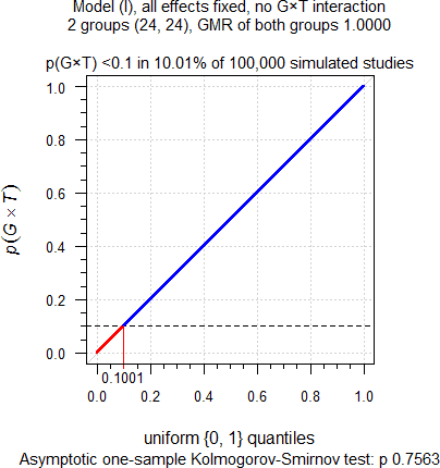
Fig. 4 No true
Group-by-Treatment interaction.
As expected. Although we simulated no true Group-by-Treatment
interaction, it is detected at approximately the level of test. Hence,
these ≈10% of cases are below the upper 95% significance limit of the
binomial test (0.1016) and are definitely false
positives. When following the
FDA’s decision scheme, only one group will be assessed for
BE by model \(\small{\text{(III)}}\), compromising
power as we have seen above. Power of one group
would be only 48.6% and hence, the study falsely considered a
failure.
Theoretically \(\small{p(G\times T)}\)
should be uniformly
distributed with \(\small{\in\left\{0,1\right\}}\). As
confirmed by the nonsignificant p-value (0.7563) of the Kolmogorov–Smirnov
test, they are.
Let’s play the devil’s advocate. A true Group-by-Treatment interaction, where the T/R-ratio in one group is the reciprocal of the other. Since groups are equally sized, in an analysis of pooled data by either model \(\small{\text{(II)}}\) or \(\small{\text{(III)}}\) we will estimate T = R.
sim.GxT(CV = 0.335, theta0 = 1, target = 0.90,
        capacity = 24, mue = c(0.95, 1 / 0.95), leg = FALSE)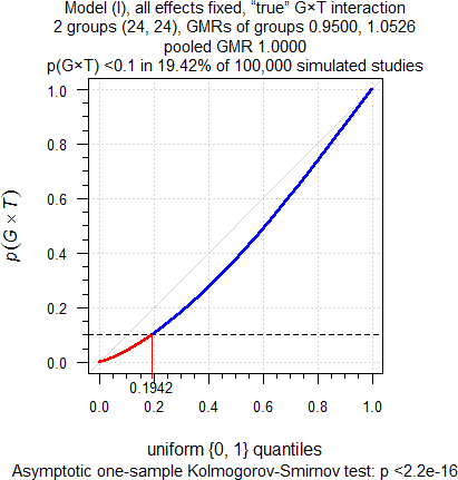
Fig. 5 True Group-by-Treatment
interaction.
As expected, again. Since there is a true Group-by-Treatment interaction, it is detected in ≈19% of cases. So far, so good. When following the FDA’s decision scheme, the T/R-ratio deviating from our assumptions will be evident because only one group will be assessed by model \(\small{\text{(III)}}\) for BE. However, in ≈81% of cases the Group-by-Treatment interaction will not be detected. That’s due to the poor power of the test. Consequently, the pooled data will be assessed by model \(\small{\text{(II)}}\) and we will estimate T = R, which is wrong because here we know that groups differ in their treatment effects. In a real study we have no clue.
Do I hear a whisper in the back row »Can’t we simply calculate the CIs of the groups and compare them?« You could, but please only at home. Since we have extremely low power, very likely the CIs will overlap. Even if not, what would you conclude? That would be yet another pre-test with all its ugly consequences. Welcome to the world of doubts.
“[The] impatience with ambiguity can be criticized in the phrase:
absence of evidence is not evidence of absence.
Not enough? Two groups (38 and 10 subjects), extreme Group-by-Treatment interaction (true T/R-ratio in the first group 1.0605 and the second 0.80, which is the Null).
sim.GxT(CV = 0.335, theta0 = 1, target = 0.90, split = c(1-10/48, 10/48),
        capacity = 40, mue = c(1.0604803726, 0.80), leg = FALSE)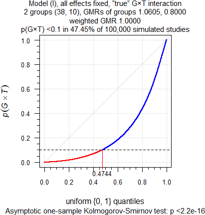
Fig. 6 Extreme true
Group-by-Treatment interaction.
Well, okay, cough… With the FDA’s decision scheme in almost 50% of cases we will evaluate only the large group and grumply accept the ≈68% power. Substantially lower than the 90% we hoped for but who cares if the study passes? Wait a minute – what about the second group? Ignore it, right? Of course, there is also a ≈50% chance that nothing suspicious will be detected and the T/R-ratio estimated as 1. No hard feelings!
Meta-study
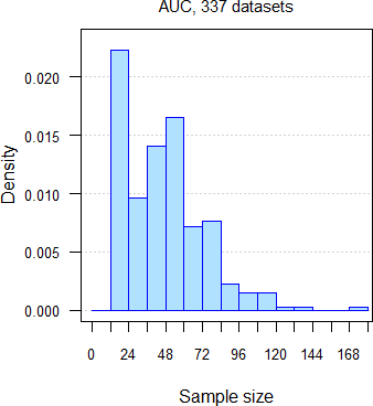
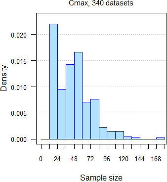
332 datasets of AUC and 335 of Cmax from 251 comparative bioavailability studies (BE, food-effect, DDI, dose-proportionality), 159 analytes, crossovers18 19 with two to seven groups, median sample size 47 subjects (15 – 176), median interval separating groups six days (one to 6220 days: ‘staggered’ approach in single dose studies and ‘stacked’ in multiple dose studies). Assessment of \(\small{\log_{e}}\)transformed PK metrics21 for the acceptance range of 80.00 – 125.00%.
Datasets were assessed for the Group-by-Treatment interaction by model \(\small{\text{(I)}}\). At a recent BE workshop22 I had a conversation with a prominent member of the FDA. She said that at the agency the Group-by-Treatment interaction is tested at the 0.05 level, thus reducing the false positive rate. Therefore, I assessed the studies at \(\small{\alpha=0.05}\). What can we expect?
- If true Group-by-Treatment interactions (p(G×T) < 0.05) exist, we would observe them in more studies than the false positive rate of the test (i.e., 0.05). Since the number of studies is limited, only > 7.23% (AUC) and > 7.16% (Cmax) would be significant.
- The distribution of p-values of the G×T-test should be standard uniform with ∈ {0, 1}. We can assess this hypothesis by the Kolmogorov–Smirnov test. In a plot p-values of studies should lie close to the unity line (running from 0|0 to 1|1).

Not representative, of course. 76.3% of datasets were single dose studies with one week or less separating groups; in 30.8% groups were separated by only one or two days. Expecting that groups could differ in their PK responses is beyond my intellectual reach.
“To consult the statistician after an experiment is finished is often merely to ask him to conduct a post mortem examination. He can perhaps say what the experiment died of.
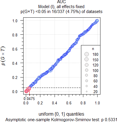
Fig. 7 332 datasets of
AUC.
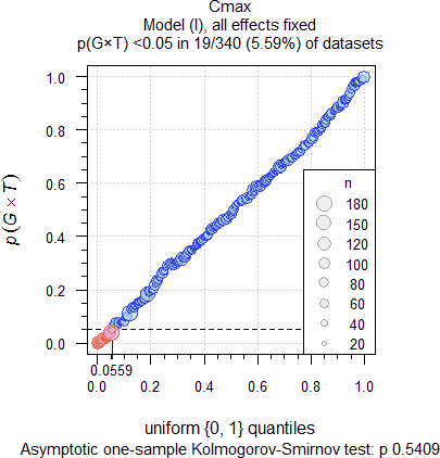
Fig. 8 335 datasets of
Cmax.
As expected, significant Group-by-Treatment interactions were
detected at approximately the level of the test (4.52% for AUC
and 5.37% for Cmax). The upper 95% significance
limits of the binomial test for n = 332 and 335 are 0.0723 and
0.0716. Hence, based on our observations in well-controlled trials
likely they are merely due to chance and can be considered ‘statistical
artifacts’, i.e., false
positives. When testing at the ‘old’ 0.1 level, we got 9.04% for
AUC and 11.04% for Cmax, again close to the
level of the test and below the respective upper limits of the binomial
test (0.1307 and 0.1295).
The Kolmogorov–Smirnov tests were not significant, accepting the
expected standard uniform distribution. Furthermore, no significant
correlations of \(\small{p(G\times
T)}\) with the sample size, number of groups, interval between
groups, and gender sex
were found.
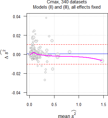
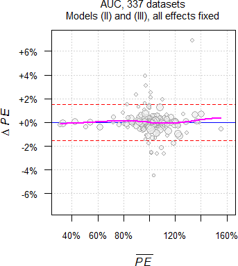
Approximately 6% less studies passed when evaluated by model \(\small{\text{(II)}}\) than by model \(\small{\text{(III)}}\). This is not only due to fewer degrees of freedom but mainly due to different residual errors (\(\small{\widehat{s^2}}\)), a finding similar to another meta-study,24 where fewer studies passed with the carryover-term in the model than without. It is impossible to predict whether the additional group-terms by model \(\small{\text{(II)}}\) can ‘explain’ part of the variability, i.e., its \(\small{\widehat{s^2}}\) may be smaller or larger than the one of model \(\small{\text{(III)}}\). \[\small{\widehat{s^2}\:\:\:\begin{array}{|lcccccccc} \textsf{metric} & \textsf{model} & \text{min.} & 2.5\% & \text{Q I} & \text{median} & \text{Q III} & 97.5\% & \text{max.}\\\hline AUC & \text{III} & \text{0.0009} & \text{0.0043} & \text{0.0134} & \text{0.0251} & \text{0.0530} & \text{0.2734} & \text{1.1817}\\ & \text{ II} & \text{0.0010} & \text{0.0042} & \text{0.0134} & \text{0.0248} & \text{0.0521} & \text{0.2774} & \text{1.1795}\\ C_\text{max} & \text{III} & \text{0.0026} & \text{0.0073} & \text{0.0296} & \text{0.0583} & \text{0.0956} & \text{0.3772} & \text{1.4657}\\ & \text{ II} & \text{0.0027} & \text{0.0074} & \text{0.0298} & \text{0.0552} & \text{0.0948} & \text{0.3768} & \text{1.4726} \end{array}}\]
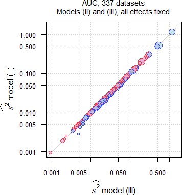
Fig. 9 Comparison of \(\small{\widehat{s^2}}\) in 332 datasets of
AUC;
blue circles where \(\small{\widehat{s^2}\,\text{(II)}\leq\widehat{s^2}\,\text{(III)}}\),
red circles where \(\small{\widehat{s^2}\,\text{(II)}>\widehat{s^2}\,\text{(III)}}\).
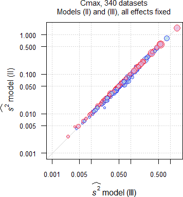
Fig. 10 Comparison of \(\small{\widehat{s^2}}\) in 335 datasets of
Cmax;
blue circles where \(\small{\widehat{s^2}\,\text{(II)}\leq\widehat{s^2}\,\text{(III)}}\),
red circles where \(\small{\widehat{s^2}\,\text{(II)}>\widehat{s^2}\,\text{(III)}}\).
In the majority of datasets (AUC ≈57%, Cmax ≈55%) \(\small{\widehat{s^2}}\) by model \(\small{\text{(II)}}\) was larger than by model \(\small{\text{(III)}}\), which is reflected in the lower passing rate. There is no dependency on the sample size.
In 1.5% of the AUC datasets and in 1.2% of the Cmax datasets the decision would change to the worse, i.e., studies passing by model \(\small{\text{(III)}}\) would fail by model \(\small{\text{(II)}}\). In none of the AUC datasets and in 1.2% of the Cmax datasets the decision would change to the better, i.e., studies failing by model \(\small{\text{(III)}}\) would pass by model \(\small{\text{(II)}}\).
As we have seen above, theoretically only \(\small{\widehat{s^2}}\) and of course, the degrees of freedom differ between models. However, in practice the Point Estimates differ as well.
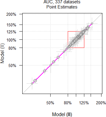
Fig. 11 Point Estimates and
their 90% CIs of 332 datasets
of AUC.
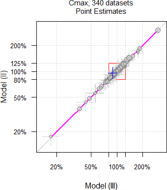
Fig. 12 Point Estimates and
their 90% CIs of 335 datasets
of Cmax.

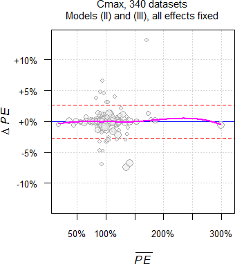
Why is that so? Currently I have no explanation. Hit by a confounder?
Let’s explore the Cmax dataset with the largest ‘bias’ we observed so far (one of only four, where the decision would change to the better).
# IBD extracted from a 6-sequence Williams design
# A = Test        (coded T)
# B = Reference 1 (coded R)
# C = Reference 2
data <- data.frame(subject = rep(1L:24L, each = 2),
                   group =  rep(1L:2L, each = 24),
                   sequence = c("CAB", "CAB", "BCA", "BCA", "CBA", "CBA",
                                "BAC", "BAC", "ABC", "ABC", "CAB", "CAB",
                                "BCA", "BCA", "BAC", "BAC", "CBA", "CBA",
                                "BCA", "BCA", "BAC", "BAC", "BCA", "BCA",
                                "ACB", "ACB", "ABC", "ABC", "CAB", "CAB",
                                "ACB", "ACB", "ABC", "ABC", "ACB", "ACB",
                                "CBA", "CBA", "CAB", "CAB", "ABC", "ABC",
                                "BAC", "BAC", "CBA", "CBA", "ACB", "ACB"),
                   treatment = c("T", "R", "R", "T", "R", "T",
                                 "R", "T", "T", "R", "T", "R",
                                 "R", "T", "R", "T", "R", "T",
                                 "R", "T", "R", "T", "R", "T",
                                 "T", "R", "T", "R", "T", "R",
                                 "T", "R", "T", "R", "T", "R",
                                 "R", "T", "T", "R", "T", "R",
                                 "R", "T", "R", "T", "T", "R"),
                   period = c(2, 3, 1, 3, 2, 3, 1, 2, 1, 2, 2, 3,
                              1, 3, 1, 2, 2, 3, 1, 3, 1, 2, 1, 3,
                              1, 3, 1, 2, 2, 3, 1, 3, 1, 2, 1, 3,
                              2, 3, 2, 3, 1, 2, 1, 2, 2, 3, 1, 2),
                   Cmax = c(41.2, 47.7, 24.2, 32.4, 19.2, 32.0,
                            43.5, 28.8, 15.4, 15.7, 29.6, 21.4,
                            40.5, 29.7, 38.5, 42.8, 52.9, 67.4,
                            32.8, 42.4, 32.6, 16.6, 25.1, 29.6,
                            16.6, 29.9, 42.2, 40.8, 42.2, 57.7,
                            40.9, 62.0, 19.1, 33.0, 35.5, 52.4,
                            51.1, 47.9, 18.4, 50.1, 30.0, 23.2,
                            30.1, 34.4, 43.0, 51.4, 23.3, 25.9))
cols       <- c("subject", "group", "sequence", "treatment", "period")
data[cols] <- lapply(data[cols], factor)
ow         <- options()
options(contrasts = c("contr.treatment", "contr.poly"), digits = 12)
model.III  <- lm(log(Cmax) ~ sequence +
                             treatment +
                             subject %in% sequence +
                             period, data = data)
MSE.III    <- anova(model.III)["Residuals", "Mean Sq"]
PE.III     <- 100 * exp(coef(model.III)[["treatmentT"]])
CI.III     <- 100 * exp(confint(model.III, "treatmentT", level = 0.9))
if (round(CI.III[1], 2) >= 80 & round(CI.III[2], 2) <= 125) {
  BE.III <- "pass"
} else {
  BE.III <- "fail"
}
model.II   <- lm(log(Cmax) ~ group +
                             sequence +
                             treatment +
                             subject %in% (group * sequence) +
                             period %in% group +
                             group:sequence, data = data)
MSE.II     <- anova(model.II)["Residuals", "Mean Sq"]
PE.II      <- 100 * exp(coef(model.II)[["treatmentT"]])
CI.II      <- 100 * exp(confint(model.II, "treatmentT", level = 0.9))
if (round(CI.II[1], 2) >= 80 & round(CI.II[2], 2) <= 125) {
  BE.II <- "pass"
} else {
  BE.II <- "fail"
}
options(ow)
res        <- data.frame(Model = c("III", "II"),
                         MSE   = signif(c(MSE.III, MSE.II), 4),
                         PE    = c(PE.III, PE.II),
                         lower = c(CI.III[1], CI.II[1]),
                         upper = c(CI.III[2], CI.II[2]),
                         BE    = c(BE.III, BE.II))
res$width <- res$upper - res$lower
res$bias  <- c(NA_real_, 100 * (res$width[2] - res$width[1]) / res$width[1])
res[, 3]  <- sprintf("%.2f%%", res[, 3])
res[, 4]  <- sprintf("%.2f%%", res[, 4])
res[, 5]  <- sprintf("%.2f%%", res[, 5])
res[, 7]  <- sprintf("%.2f%%", res[, 7])
res[2, 8] <- sprintf("%+.2f%%", res[2, 8])
res[is.na(res)] <- "   –"
print(res, row.names = FALSE, right = FALSE)
# Model MSE PE lower upper BE width bias
# III 0.05392 89.10% 79.38% 100.02% fail 20.64% –
# II 0.05337 96.06% 82.91% 111.28% pass 28.37% +37.48%Although \(\small{\widehat{s^2}}\) of model \(\small{\text{(II)}}\) is only marginally smaller than the one of model \(\small{\text{(III)}}\) (CVw 23.4% vs 23.5%), the ‘better’ Point Estimate would save the study (see Fig. 12 in blue).
It can by a close shave:
In one of the AUC datasets (18 subjects in each of two groups
and 17 in one) \(\small{\widehat{s^2}}\) increased from
0.07130 by model \(\small{\text{(III)}}\) to 0.07395 by
model \(\small{\text{(II)}}\). Together with 49
degrees of freedom instead of 51, the 90%
CI is 104.81 – 125.13% instead
of 104.97 – 124.90%. Hence, the study would fail by model \(\small{\text{(II)}}\), though it passed
by model \(\small{\text{(III)}}\).
Not close
enough? In one of the Cmax datasets (38 and 36
subjects / group) the study passed with the 90%
CI of 98.99 – 124.92% by
model \(\small{\text{(III)}}\) but would fail
with 98.96 – 125.09% by model \(\small{\text{(II)}}\).
In both
cases \(\small{p(G\times T)}\) were not
significant (0.5390, 0.7146) but lead to deficiency letters requesting
evaluation by model \(\small{\text{(II)}}\). I don’t know the
outcome…
Especially in multi-site studies model \(\small{\text{(II)}}\) may recover
information indeed. In one case (three subjects in two sites, four,
five, and 14 subjects in three others) \(\small{\widehat{s^2}}\) of
Cmax decreased substantially from 0.2677 by model \(\small{\text{(III)}}\) to 0.1630 by
model \(\small{\text{(II)}}\). The study
would have passed with an upper
CL of 110.49% but was a complete
disaster with 149.03% according to the protocol – ignoring the
multi-site structure.
Quoting a Swedish inspector: »Don’t worry, it’s
too late.«
Fake Groups
AUC data from the literature.27 54 subjects, four period full replicated design. I assessed only the 52 subjects with complete data (excluded #3 and #27). I randomly allocated subjects to two ‘fake groups’ (12 – 40 subjects) and assessed the \(\small{G\times T}\) test. Below only significant results where the ‘fake groups’ had similar sizes.
data <- data.frame(subject = c(rep(1L:2L, each = 4), rep(3L, 2),
                               rep(4L:13L, each = 4), rep(15L:26L, each = 4),
                               rep(27L, 2), rep(28L:40L, each = 4),
                               rep(42L:50L, each = 4), rep(52L:57L, each = 4)),
                   period = c(rep(1L:4L, 2), 1L:2L, rep(1L:4L, 10),
                              rep(1L:4L, 12), 1L:2L, rep(1L:4L, 13),
                              rep(1L:4L, 9), rep(1L:4L, 6)),
                   sequence = c(rep("RTRT", 4), rep("TRTR", 4), rep("RTRT", 2),
                                rep("TRTR", 4), rep("RTRT", 8), rep("TRTR", 12),
                                rep("RTRT", 4), rep("TRTR", 4), rep("RTRT", 4),
                                rep("TRTR", 4), rep("RTRT", 4), rep("TRTR", 4),
                                rep("RTRT", 8), rep("TRTR", 8), rep("RTRT", 4),
                                rep("TRTR", 8), rep("TRTR", 8), rep("TRTR", 6),
                                rep("RTRT", 8), rep("TRTR", 4), rep("RTRT", 4),
                                rep("TRTR", 8), rep("RTRT", 8), rep("TRTR", 12),
                                rep("RTRT", 8), rep("TRTR", 8), rep("RTRT", 4),
                                rep("TRTR", 4), rep("RTRT", 4), rep("TRTR", 4),
                                rep("RTRT", 12), rep("TRTR", 4), rep("RTRT", 8),
                                rep("TRTR", 8), rep("RTRT", 4)),
                   treatment = NA_character_, group = NA_integer_,
                   AUC = c(812.6, 1173.7, 889.1, 620.1, 216.3, 338.0, 502.8,
                           398.6,  545.1, 542.9, 632.6, 520.0, 716.7, 860.4,
                           400.0,  223.8, 173.7, 289.7, 102.1, 185.3,  42.0,
                            88.3,  596.0, 659.3, 543.8, 662.9, 402.4, 359.8,
                           590.8,  444.3, 456.7, 378.4, 477.5, 407.9, 304.5,
                           351.5,  520.2, 335.7, 500.7, 323.0, 416.3, 525.1,
                           176.1,  710.7, 409.5, 645.5, 160.6, 218.0, 170.1,
                           124.6,  562.4, 490.4, 504.7, 675.9, 756.0, 606.8,
                           477.4,  626.8, 207.5, 271.6, 173.7, 240.5, 571.3,
                           705.2,  619.0, 633.6, 511.9, 549.7, 388.2, 141.0,
                           124.0,   91.9, 113.3,  59.5, 536.1, 595.2, 445.5,
                           521.5,  239.7, 265.1, 445.9, 433.2, 609.6, 371.6,
                           511.3,  432.7, 449.9, 860.4, 606.8, 577.2, 192.5,
                           220.1,  233.1, 227.0, 764.4, 508.8, 757.8, 449.4,
                           151.9,  194.8, 568.1, 321.1, 338.3, 403.6, 735.6,
                           634.5, 1244.2, 641.9, 429.1, 391.8, 316.9, 335.1,
                           307.4,  481.8, 346.6, 369.7, 409.0, 514.6, 763.1,
                           406.5,  271.0, 221.0, 296.5, 463.7, 292.9, 431.0,
                           448.5,  267.8, 217.2, 332.2, 103.0, 127.5, 290.8,
                           208.6,  243.7, 489.7, 297.2, 502.0, 320.4, 334.3,
                           163.8,  232.1, 636.9, 434.9, 368.3, 292.6, 446.1,
                           222.3,  193.7, 202.8, 255.2, 244.3, 534.1, 243.1,
                           418.4,  441.9, 355.1, 415.2, 382.7, 334.0, 102.0,
                           282.5,  245.6, 286.2, 320.5, 233.9, 331.7, 260.5,
                           223.6,  645.4, 349.0, 507.4, 504.5, 289.9, 550.7,
                           244.2,  615.8, 732.1, 620.9, 665.2, 898.4, 924.9,
                           398.3,  828.3, 410.4, 329.2, 449.4, 442.1, 237.0,
                           505.0,  496.3, 580.6, 332.4, 273.6, 525.3, 293.3,
                           185.2,  222.9, 182.1, 194.1, 246.9, 620.9, 678.3,
                           752.2,  235.4, 190.4, 318.3, 248.4, 180.6, 174.7,
                           102.9,  117.0))
for (i in 1:nrow(data)) {# extract treatments from sequences and periods
  treatments        <- unlist(strsplit(data$sequence[i], split = ""))
  data$treatment[i] <- treatments[data$period[i]]
}
subj <- unique(data$subject)
keep <- numeric(0)        # keep only subjects with complete data
for (i in seq_along(subj)) {
  tmp <- data[data$subject == subj[i], 2]
  if (length(data$period[data$subject == subj[i]]) == 4) keep[i] <- subj[i]
}
keep             <- keep[!is.na(keep)]
data             <- data[data$subject %in% keep, ]
n.subj           <- as.integer(length(unique(data$subject)))
data$subject     <- rep(1L:n.subj, each = 4) # easier
facs             <- c("subject", "sequence", "treatment", "period", "group")
ow               <- options()
options(contrasts = c("contr.treatment", "contr.poly"), digits = 12)
nsims            <- 2500L
res              <- data.frame(n.grp1 = rep(NA_integer_, nsims),
                               n.grp2 = NA_integer_,
                               p.GxT = NA_real_, sig = FALSE)
set.seed(123456)
n.grps           <- round(runif(n = nsims, min = 12, max = n.subj - 12))
for (i in 1:nsims) {
  tmp           <- data
  select        <- round(runif(n = n.grps[i], min = 12, max = n.subj - 12))
  res$n.grp1[i] <- n.grps[i]
  res$n.grp2[i] <- n.subj - res$n.grp1[i]
  tmp$group     <- 2L
  tmp$group[tmp$subject %in% select] <- 1L
  tmp[facs]     <- lapply(tmp[facs], factor)
  model1        <- lm(log(AUC) ~ group +
                                 sequence +
                                 treatment +
                                 subject %in% (group*sequence) +
                                 period %in% group +
                                 group:sequence +
                                 group:treatment, data = tmp)
  res$p.GxT[i]  <- anova(model1)[["group:treatment", "Pr(>F)"]]
}
options(ow)
res                      <- unique(res)
res$sig[res$p.GxT < 0.1] <- TRUE
res$p.GxT                <- round(res$p.GxT, 6)
res                      <- res[with(res, order(p.GxT, n.grp1)), ]
print(res[res$n.grp1 >= 25 & res$n.grp1 <= 27 &
          res$n.grp2 >= 25 & res$n.grp2 <= 27 &
          res$sig == TRUE, ], row.names = FALSE)
# n.grp1 n.grp2 p.GxT sig
# 27 25 0.025003 TRUE
# 25 27 0.033413 TRUE
# 27 25 0.058473 TRUE
# 25 27 0.063708 TRUE
# 26 26 0.072094 TRUE
# 27 25 0.076887 TRUE
# 25 27 0.085086 TRUE
# 26 26 0.090428 TRUE
# 27 25 0.091810 TRUE
# 27 25 0.095832 TRUE5.04% of cases showed a significant Group-by-Treatment
interaction.
Recall: The study was not performed in groups! Hit by Murphy.
Summary
In multi-site studies always model \(\small{\text{(II)}}\) should be employed. For details see section 3.2 of ICH E9.28 Recently the FDA and the ICH recommended it for multi-group studies as well.5 6
- The FDA’s decision scheme based on the above is only given for multi-group
studies. When it comes to multi-site studies, how should we
interpret »questions may arise as to whether the results from the
several groups should be combined in a single analysis«?
Cave: Intra-subject contrasts for the estimation of the treatment effect (and hence, the PE and its CI) cannot be unbiased obtained from model (I).13 The G × T test serves only as a tool in the decision scheme. - If model (I) is performed as a pre-test, it inflates
the family-wise
error rate (i.e., the probability α of the Type I
Error, the consumer risk ) and hence, its application is
statistically flawed from the start. Well known examples where
a pre-test inflates the Type I Error are testing for an unequal
carryover effect in crossover studies29 (see also this article) and
assessing variance
homogenicity in parallel designs.30
- Even if there is a true Group-by-Treatment interaction, it will not be detected in the majority of cases and hence, application of model (II) questionable.
- As shown in the simulations, power of the G × T test is poor. If there is no true Group-by-Treatment interaction, it will be falsely detected in ~10% of cases, seriously compromising power.
- The FDA tests
the Group-by-Treatment interaction at the 0.05 level,22 thus reducing the false positive rate (in the
meta-study we got 4.52% for AUC and 5.37%
for Cmax instead of 9.04% for AUC and
11.04% for Cmax if tested at the 0.1 level). That’s
good, but then the member of the
FDA also said
»We often see not only p-values just below 0.05, but also some with 0.0001 and lower…«It’s a common fallacy to regard the p-value as the probability that the Null Hypothesis is true (or the Alternative Hypothesis is false).31 In frequentist statistics the outcome of any level α-test is dichotomous: Hypotheses are considered true or false, not something that can be represented with a probability (see also this article).
- »[…] it may not be necessary […]« leaves room for interpretation.
- Similar demographics are not relevant in crossover studies, since each subject acts as its own reference. In parallel designs such a requirement is trivial (applicable to single group-/site-studies as well).
- Should »one of the groups« be understood as the largest one? It is unclear how to proceed if there are equally sized groups. Most conservative would be to follow the intersection-union principle32 and require demonstration of BE in all of them, although this will be quite restrictive.
“It is not a requirement that each group separately pass the confidence interval requirement. […] if at least one of the groups individually passes the confidence interval criteria, then the test product would be acceptable.
[…] if the groups are studied at the same location under the identical protocol, and there is overlap in time among the treatments given to the different groups, as occurs often, there may be no obvious reason for a significant interaction. Perhaps, the result was merely due to chance, random variation. One may then present an argument for accepting the pooled results.
I’m a bit skeptic. The larger the group, the more reliable the outcome will be. What if a small group passes – by chance – and all others fail?
Essentially, a statement in the context of the ‘sequence effect’ is applicable here as well.
“Testing for carryover in bioequivalence studies […] is not recommended and, moreover, can be harmful. It seems that whenever carry-over is ‘detected’ under such conditions, it is a false positive and researchers will be led to use an inferior estimate, abandoning a superior one.
North American CROs routinely evaluate \(\small{\text{(I)}}\) with no consequences if the \(\small{G\times T}\) test is significant, i.e., for the assessment of BE model \(\small{\text{(II)}}\) is used. Very few deficiency letters issued by the FDA. Most we have seen so far were received by European CROs. Politics?
“All animals are equal, but some animals are more equal than others.
Good news from the other side of the pond: The FDA accepted in a ‘Type A’ meeting in April 2021 our arguments, especially about the inflated Type I Error.35 Hence, the FDA conceded that for our study the pre-test \(\small{\text{(I)}}\) in the decision scheme is not required and \(\small{\text{(II)}}\) can be used. This is also reflected in the recent draft guidance.5
Given the outcome of the small meta-study, significant Group-by-Treatment interactions are most likely false positives. To avoid problems with the FDA, in some MENA-states (especially Saudi Arabia), the EEU, and recently with some European assessors, we recommend to opt for model \(\small{\text{(II)}}\) in any case. The impact on power compared to the conventional model \(\small{\text{(III)}}\) is acceptable and its application avoids lengthy and fruitless discussions.
In the context of Two-Stage Designs the EMA stated in the Q&A document:36
“Discussion
A model which also includes a term for a formulation*stage interaction would give equal weight to the two stages, even if the number of subjects in each stage is very different. The results can be very misleading hence such a model is not considered acceptable. Furthermore, this model assumes that the formulation effect is truly different in each stage. If such an assumption were true there is no single formulation effect that can be applied to the general population, and the estimate from the study has no real meaning.
Conclusion
3) A term for a formulation*stage interaction should not be fitted.
On another note: None of the published TSD-methods contains a test of ‘poolability’. In responding deficiency letters, we successfully replaced ‘stage’ by ‘group’.
According to the FDA’s recently revised guidance5 and the ICH’s draft guideline:6
“Bioequivalence should be determined based on the overall treatment effect […] the assessment of BE in the whole study population should be done without including the treatment and group interaction(s) term in the model.
In a deficiency letter of 201837 related to a multi-site study of a biosimilar (\(\small{\text{I}}\) → \(\small{\text{III}}\)) the EMA stated:
- A sub-set of patients cannot be selected for the BE analysis on the basis of tests for a treatment-by-site interaction. It is questioned whether this approach produces an unbiased estimate as the chosen group may no longer be representative of the initial intended study population. The Type I error is not controlled when the procedure […] is only related to the finally selected population / model.
- In a multi-site study Model II is preferred, and that should be used for the BE analysis regardless of the results of any interaction tests.
Interpreting the guidelines:3 6
»Can [it] be reasonably assumed«
that in a study with identical in- and exclusion criteria, similar demographic characteristics across groups, performed in the same CRO, quite often groups separated by only a couple of days, samples analyzed with the same bioanalytical method in the same lab, in a crossover each subject acting as its own reference,
»have an effect on the response variable«‽
Of course, not. IMHO, assuming the opposite is an insult to the mind.
»Λόγον ἔχεις;« »ἔχω.« »τί οὖν οὐ χρᾷ;«
‘Hast thou reason?’ ‘I have.’ ‘Why then makest thou not use of it?’
Therefore, the conventional model \(\small{\text{(III)}}\) could be used (without a justification). In 40+ years I came across only two cases where model \(\small{\text{(II)}}\) was requested by a European agency (one multi-group and one multi-site study). When I gave a presentation38 about groups/sites in BE in front of European regulatory (‼) statisticians, they were asking in disbelieve »What the heck are you talking about?«
However, never say never…
NB, the size of the second group was just 6% of the first. The 90% CI of Cmax was 87.96 – 100.93% by model \(\small{\text{(III)}}\) and 87.88 – 101.37% by \(\small{\text{(II)}}\).
Did the assessor expect that the study would suddenly fail, only because there is one degree of freedom less? Or was he/she worried about the one day separating groups?
In another, also of 2021:
It was a four-period full replicate design (Cmax by ABEL, AUCt by ABE) in the staggered approach and groups were separated by two days. There were 46 subjects in one group and 14 in the other. Even the larger one was underpowered and hence, failed on AUCt.
An example of 2022:
An FDC product with two APIs, PK metrics AUCτ,ss, Cmax,ss, and Cτ,ss. The study was performed in two groups (31 and 28 eligible subjects); passed BE per protocol by model \(\small{\text{(III)}}\) and would have passed by model \(\small{\text{(II)}}\) as well.
- A European [sic] agency asked for assessment of the Group-by-Treatment interaction. One of the six tests (Cτ,ss of one API) was significant (p 0.03). Not astonishing with the \(\small{G\times T}\) test’s false positive rate of 10%…
-
The arguments of the applicant were not accepted. Instead, the agency
asked for separate evaluation of groups. All
PK metrics passed, except
Cτ,ss in the smaller
group, which failed by a small margin (78.76%).
Two APIs × three PK metrics × two groups = whopping twelve comparisons…
What’s the point? Of course, the study was powered for model \(\small{\text{(III)}}\) and the
applicant was extremely lucky39 that the other
PK metrics passed in the separate
evaluations with roughly only half the planned sample size in both
groups.
As an aside, the same drug was studied in single dose studies
(fasting/fed) as well. No significant Group-by-Treatment interaction of
Cmax and AUC0–t. Hence, overall
there was a single [sic] significant \(\small{G\times T}\) test out of
14.
Discussions with the agency are ongoing. Outright bizarre. What a
waste of time!
Hot off the press (2023):
Amazing, yet another variant!
Perhaps the agencies had a crystal ball because these deficiency letters (except the last) were in line with the ICH’s draft guideline:6
“[…] the appropriateness of the statistical model should be evaluated to account for the multi-group nature of the BE study.
Smells of model \(\small{\text{(II)}}\), right? However, the guideline continues:
“Applicants should evaluate potential for heterogeneity of treatment effect across groups, i.e., Group by Treatment interaction. If the Group by Treatment interaction is significant, this should be reported and the root cause of the Group by Treatment interaction should be investigated to the extent possible. Substantial differences in the treatment effect for PK parameters across groups should be evaluated. Further analysis and interpretation may be warranted in case heterogeneity across groups is observed.
 © 2008 hobvias sudoneighm
@ flickr
© 2008 hobvias sudoneighm
@ flickr
Oh dear, that calls for model \(\small{\text{(II)}}\) and – subsequently – model \(\small{\text{(I)}}\)!
- Which significance level of the G × T test should be applied? 0.1 like in our simulations or the less restrictive 0.05 used by the FDA (see above)?
- What on earth could be the root cause of something happening by chance? Only dark magic could answer this question.
- As we have seen, statistics cannot help at all. What extent of investigation is considered possible? If an agency is concerned about fraud (see above), it should initiate an inspection to satisfy its paranoid curiosity – without burdening the sponsor or CRO (recall that we are talking about ~10% of studies performed in groups).
- Which differences in the treatment effect […] across groups might be regarded as substantial by assessors?
- If all pairwise comparisons are considered (our understanding of ‘across groups’), their number increases quickly with the number of groups, e.g., with four groups (assessing AUC and Cmax) we have already twelve…40
- What kind of further analysis did the authors have in mind?
- This section opens the door to lenghty – and likely fruitless – discussions. Already interpretation is a misnomer.
“The combination of some data and an aching desire for an answer does not ensure that a reasonable answer can be extracted from a given body of data.
“A mathematician is a blind man in a dark room looking for a black cat which isn’t there.
To our knowledge only one publication explored different models for multi-group studies.41 While the authors recommend a mixed-effects model, according to guidelines in 2×2×2 crossover studies only complete data should be used. We don’t agree with the authors that ‘group’ should be treated as a random effect, unless an additional group was recruited to counteract the loss in power due to dropouts.
Recommendations
Like in testing for unequal carryover (aka the ‘sequence effect’, see this article) a statistical ‘correction’ of a true Group-by-Treatment interaction is not possible. One can only try to avoid problems by design.
- The FDA’s
former decision scheme model (I) → model (II) or model (III) is not
appropriate and hence, should be avoided.
- Due to the low power of the test (based on a between-subject factor), in the majority of cases a true Group-by-Treatment interaction will not be detected.
- Power is compromised and – more importantly – the Type I Error inflated.
- If a study is performed in multiple groups, model (II) is recommended,
except for the
FDA and in the
EEU, where it is mandatory.
For Japan’s
NIHS model
(III) is
acceptable under certain conditions
(e.g., the sizes of groups should be similar). The
FDA recommends
similar group sizes as well, although it is not one of the four
mandatory conditions.
- In single dose studies groups should be dosed in the ‘staggered’ approach and in multiple dose studies in the ‘stacked’ approach.
- All subjects should be recruited from the same enrollment pool.
- If a study is performed in multiple sites, model (II) is mandatory.
- In-/exclusion criteria should be identical across sites.
In either case:
- All enrolled subjects should be randomly assigned to treatments at study outset.
- Samples should be analyzed by the same bioanalytical method in the same lab.
- The model must be unambiguously stated in the protocol.
- Based on the observations in the small meta-study up to 7% power may be lost in multi-group studies by model (II) and hence, the sample size increased accordingly.
top of section ↩︎ previous section ↩︎
Acknowledgment
The 27 companies and individuals of 17 countries for providing data for the meta-analysis.
Anders Fuglsang (Fuglsang Pharma, Vejle Ø, Denmark), Jiří Hofmann (Zentiva, Prague, Czech Republic), Detlew Labes (consultant, Berlin, Germany), Barbara Schug (SocraTec, Oberursel, Germany), Anastasia Shitova (Quinta Analytica, Yaroslavl, Russian Federation), Volodymyr Stus (Polpharma, Gdańsk, Poland), Michael Tomashevskiy (OnTarget Group, Saint Petersburg, Russian Federation), and Ralph-Steven Wedemeyer (SocraTec, Oberursel, Germany), as well as users ‘zan’ and ‘zizou’ of the BEBA-Forum for fruitful discussions.
Postscript
We are still collecting data for the meta-study.
Of course, data will be treated strictly confidential
and not published. The preferred format of flat-files
is CSV
(although XLS(X),
ODS, XPT,
or Phoenix project files would do as well).
Please send data to [email protected]
or [email protected].
| # | Column | Format | Description |
|---|---|---|---|
| 1 |
Source
|
text | Name of company, CRO, or individual providing the data |
| 2 |
Code
|
text | Any identifier of the study |
| 3 |
Analyte
|
text |
If you don’t want to disclose this information, use
not spec. X, where X is an integer
1 … number of analytes
|
| 4 |
Design
|
2x2 | Simple crossover |
| 3x6x3 | 6-sequence 3-period Williams’ design | ||
| 3x3 | 3-period Latin Squares | ||
| 4x4 | 4-sequence 4-period Williams’ design or 4-period Latin Squares | ||
| 2x2x4 | 2-sequence 4-period full replicate | ||
| 2x2x3 | 2-sequence 3-period full replicate | ||
| 2x3x3 | 3-sequence 3-period (partial) replicate | ||
| 2x4x2 | 4-sequence 2-period full replicate (Balaam’s design) | ||
| 5 |
Drug
|
integer |
1 … number of analytes
|
| 6 |
Subject
|
integer or text | Must be unique |
| 7 |
Group or Site
|
integer or text |
1 … the number of groups or sites
|
| 8 |
Sequence
|
integer or text |
Essentially any kind of coding is possible, as long as it is
unambiguous, e.g., TR, RT or
AB, BA or 1, 2
(simple crossover), ABC, BCA, CAB
(Latin Squares), ABC, ACB, BAC,
BCA, CAB, CBA (Williams’ design),
TRTR, RTRT or TRT,
RTR (full replicate designs), TRR,
RTR, RRT (partial replicate design),
TR, RT, TT, RR
(Balaam’s design)
|
| 9 |
Treatment
|
character |
Mandatory T or R (not A
or B)
|
| 10 |
Period
|
integer |
1 … number of periods
|
| 11 |
AUC
|
numeric |
For single dose AUC0–t or
AUC0–72, for multiple dose AUC0–τ Missing values should be coded with NA (preferred) or Missing
|
| 12 |
Cmax
|
numeric | For single dose Cmax, for multiple dose Css,max |
| 13 |
Interval
|
integer | Days separating groups; only if equal across groups |
| 14 |
Sex
|
character |
f or m
|
Columns 1–12 are mandatory and 13–14 optional (although desired). Any
order of columns is acceptable. Rows can be given in any order. The
evaluation script will sort them by
Source–Code–Drug–Group–Subject–Period.
Example
Source Code  Analyte  Design Drug Subject Group Sequence Treatment Period AUC Cmax
 CROX  S123 Ibuprofen  2x2    1      1      1      TR        T        1   425 45.3
 CROX  S123 Ibuprofen  2x2    1      1      1      TR        R        2   447 50.3
...
 CROX  S123 Ibuprofen  2x2    1     25      2      RT        R        1   402 47.3
 CROX  S123 Ibuprofen  2x2    1     25      2      RT        T        2   383 40.8
...
No cherry-picking, otherwise we will fall into the trap of selection bias
and the outcome will be useless. Hence, if you decide to provide data,
please do so irrespective of whether you ‘detected’ a significant
Group-by-Treatment interaction or not. We are primarily working on 2×2×2
crossover designs. However, if you have data of replicate designs, fine
as well. In Higher-Order crossover designs indicate which of the
treatments is the test and which the reference.
If possible, give the analyte. Once we have enough datasets, we may
perform sub-group analyses.
So far we have only one multi-site study. If you could share some data, great.
Post postscript
Out of curiosity I had a ‘conversation’ with ChatGPT.
Q
“Is it acceptable to perform a crossover bioequivalence study in multiple groups?
A
“It is generally not acceptable to perform a crossover bioequivalence study in multiple groups, as this can introduce additional sources of variability and increase the risk of bias in the study.
In a crossover study, each subject serves as his or her own control, receiving both the test and reference treatments in a randomized sequence. This design is intended to minimize inter-subject variability and increase the precision of the estimates of bioequivalence.
If multiple groups are used in a crossover study, each group would receive a different randomization sequence, which could result in differences in the bioavailability of the drug between the groups due to factors such as residual carryover effects, differences in diet, or differences in subject characteristics.
In general, a crossover study should be performed in a single group of subjects, with each subject receiving both the test and reference treatments in a randomized sequence. This design allows for the assessment of within-subject variability and provides a more accurate estimate of bioequivalence.
However, there may be situations where a multiple-group crossover study is appropriate, such as in studies of drugs with known ethnic differences in pharmacokinetics. In such cases, careful consideration should be given to the study design and statistical analysis plan to minimize bias and ensure that the results are interpretable.
Licenses
 Helmut Schütz 2024
R and PowerTOST GPL 3.0,
klippy MIT,
pandoc GPL 2.0.
1st version July 29, 2022. Rendered May 3, 2024 16:41 CEST by
rmarkdown via
pandoc in 0.33 seconds.
Footnotes and References
Labes D, Schütz H, Lang B. PowerTOST: Power and Sample Size for (Bio)Equivalence Studies. Package version 1.5.6. 2024-03-18. CRAN.↩︎
FDA, CDER. Guidance for Industry. Statistical Approaches to Establishing Bioequivalence. Rockville. January 2001. Download.↩︎
EMA, CHMP. Guideline on the Investigation of Bioequivalence. London. 20 January 2010. Online.↩︎
Council of the EEC. On the approval of the rules for conducting research of bioequivalence of drugs within the framework of the EEU. November 3, 2016; amended September 4, 2020.↩︎
FDA, CDER. Draft Guidance for Industry. Statistical Approaches to Establishing Bioequivalence. Silver Spring. December 2022. Revision 1. Download.↩︎
ICH. Bioequivalence for Immediate Release Solid Oral Dosage Forms. M13A. Draft version. 20 December 2022. Online.↩︎
Statisticians may be more familiar with the terminology \(\small{\textrm{AB}|\textrm{BA}}\).
Forgive me – in bioequivalence \(\small{\textrm{TR}|\textrm{RT}}\) is commonly used, where \(\small{\textrm{T}}\) denotes the Test and \(\small{\textrm{R}}\) the Reference treatment (formulation).↩︎Bolton S, Bon C. Pharmaceutical Statistics. Practical and Clinical Applications. New York: informa healthcare; 5th ed. 2010. p. 629.↩︎
If Subject 1 is randomized to sequence \(\small{\text{TR}}\), there is not ‘another’ Subject 1 randomized to sequence \(\small{\text{RT}}\). Randomization is not like Schrödinger’s cat. Hence, the nested term in the guidelines is an insult to the mind.↩︎
NIHS, Division of Drugs. English translation of Attachment 1 of PSEHB/PED Administrative Notice. March 19, 2020. Online. Original [Japanese].↩︎
In the literature you may find the term ‘Geometric Means Ratio’ (GMR) instead, which is equivalent to the one used in \(\small{(4)}\) because:
\(GMR=\frac{GM_{\text{x}_\text{T}}}{GM_{\text{x}_\text{R}}}=\frac{\sqrt[n_\text{T}]{\prod x_\text{T}}}{\sqrt[n_\text{R}]{\prod x_\text{R}}}=\frac{\left(\prod x_\text{T}\right )^{\tfrac{1}{n_\text{T}}}}{\left(\prod x_\text{R}\right )^{\tfrac{1}{n_\text{R}}}}=\frac{\sum \log_{e}x_\text{T}}{n_\text{T}}-\frac{\sum \log_{e}x_\text{R}}{n_\text{R}}=\overline{\log_{e}x_\text{T}}-\overline{\log_{e}x_\text{R}}\:\square\)↩︎FDA, CDER. ANDA 077570. Bioequivalence Reviews. 2008. Control document #98-392 regarding the Group-by-Treatment interaction discussion. September 10, 1999. Online.↩︎
WHO. Frequent deficiencies in BE study protocols. Geneva. November 2020. Online.↩︎
Quoting my late father: »If you believe, go to church.«↩︎
Alosh M, Fritsch K, Huque M, Mahjoob K, Pennello G, Rothmann M, Russek-Chen E, Smith E, Wilson S, Yiu L. Statistical Considerations on Subgroup Analysis in Clinical Trials. Stat Pharm Res. 2015; 7(4): 286–304. doi:10.1080/19466315.2015.1077726.↩︎
Schütz H, Burger DA, Cobo E, Dubins D, Farkas T, Labes D, Lang B, Ocaña J, Ring A, Shitova A, Stus V, Tomashevskiy M. (in press). Group-by-Treatment Interaction Effects in Comparative Bioavailability Studies. AAPS J.↩︎
Sagan C. The Demon-Haunted World: Science as a Candle in the Dark. New York: Random House; 1995. Ch. 12. The Fine Art of Baloney Detection.↩︎
Why so few? If ever possible my clients try to avoid multi-group and multi-site studies – and for a reason. More datasets than studies because some were FDC products with multiple analytes or IBDs extracted from Williams’ designs.
I have data of studies of my old CRO on file, which – given the sample size and clinical capacity – were definitely performed in groups. Since evaluation by model \(\small{\text{(III)}}\) was the standard back in the day, the data don’t contain information about groups. Regrettably I don’t have the clinical reports.↩︎253 2×2×2 designs, 33 two-sequence four-period full replicate designs, three partial replicate design, as well as 46 IBDs (for the ‘Two at a Time’ approach) extracted from six-sequence three-period and four-sequence four-period Williams’ designs. More datasets than studies due to multiple analytes in FDC products or metabolites additionally to the parent drug.↩︎
Unplanned interruption due to COVID-19 restrictions. Next longest interval 18 days.↩︎
In single dose studies AUC0–t or AUC0–72 and Cmax, in multiple dose studies AUC0–τ and Css,max.↩︎
Medicines for Europe. 2nd Bioequivalence Workshop. Session 2 – ICH M13 – Bioequivalence for IR solid oral dosage forms. Brussels. 26 April 2023.↩︎
Fisher RA. Presidential Address to the First Indian Statistical Congress. Sankhya. 1938; 4: 14–7.↩︎
D’Angelo G, Potvin D, Turgeon J. Carry-over effects in bioequivalence studies. J Biopharm Stat. 2001; 11(1&2): 35–43. doi:10.1081/bip-100104196.↩︎
Bland JM, Altman DG. Measuring agreement in method comparison studies. Stat Methods Med Res. 1999; 8(2): 135–60. doi:10.1177/096228029900800204.↩︎
Cleveland WS, Grosse E, Shyu WM. Local regression models. In: Chambers JM, Hastie TJ, editors. Statistical Models in S. New York: Routledge; 1992. doi:10.1201/9780203738535. Chapter 8.↩︎
Patterson SD, Jones B. Bioequivalence and statistics in clinical pharmacology. Boca Raton: CRC Press; 2nd ed. 2017. Table 4.30. pp. 105–6.↩︎
ICH. Statistical Principles for Clinical Trials. E6. 5 February 1998. Online.↩︎
Freeman PR. The performance of the two-stage analysis of two-treatment, two-period crossover trials. Stat Med. 1989; 8(12): 1421–32. doi:10.1002/sim.4780081202.↩︎
Zimmerman DW. A note on preliminary tests of equality of variances. Br J Math Stat Psychol. 2004; 57(1): 173–81. doi:10.1348/000711004849222.↩︎
Wasserstein RL, Lazar NA. The ASA’s Statement on p-Values: Context, Process, and Purpose. Am Stat. 2016; 70(2): 129–33. doi:10.1080/00031305.2016.1154108.
 Open
Access.↩︎
Open
Access.↩︎Berger RL, Hsu JC. Bioequivalence Trials, Intersection-Union Tests and Equivalence Confidence Sets. Stat Sci. 1996; 11(4): 283–302. JSTOR:2246021.↩︎
Senn S, D’Angelo G, Potvin D. Carry-over in cross-over trials in bioequivalence: theoretical concerns and empirical evidence. Pharm Stat. 2004; 3: 133–42. doi:10.1002/pst.111.↩︎
Orwell G. Animal Farm. A Fairy Story. London: Secker and Warburg; 1945.↩︎
Schütz H. Multi-Group Studies in Bioequivalence. To pool or not to pool? Presentation at: BioBridges. Prague. 26–27 September 2018. Online.↩︎
EMA, CHMP. Questions & Answers: positions on specific questions addressed to the Pharmacokinetics Working Party (PKWP). Rev. 13. London. 19 November 2015 (originally published in Rev. 7. 13 February 2013). Online.↩︎
Before you ask: Sorry folks, that’s confidential. 😎 ↩︎
Schütz H. Multi-Group and Multi-Site Studies. To pool or not to pool? 2nd Annual Biosimilars Forum. Satellite Short Course. Budapest. 5 October 2017. Online.↩︎
T/R-ratios and CVs were ‘better’ than assumed, as well as the dropout-rate lower than anticipated in the sample size estimation.↩︎
Let \(\small{n}\) be the number of groups and \(\small{p}\) the number of PK-metrics. Then the number of pairwise comparisons is given by \(\frac{n!}{2\,(n-2)!}\times \small{p}\). In the most extreme case of our meta-study (117 subjects in seven groups; AUC and Cmax) that would call for 42 (forty-two‼) comparisons.↩︎
Bae K-S, Kang S-H. Bioequivalence data analysis for the case of separate hospitalization. Transl Clin Pharmacol. 2017; 25(2): 93–100. doi:10.12793/tcp.2017.25.2.93.
Open
Access.↩︎