Consider allowing JavaScript. Otherwise, you have to be proficient in reading LaTeX since formulas will not be rendered. Furthermore, the table of contents in the left column for navigation will not be available and code-folding not supported. Sorry for the inconvenience.

Examples in this article were generated with 4.2.1 by the packages PowerTOST,¹ lattice,² and latticeExtra³ on Windows 7 build 7601, Service Pack 1, Universal C Runtime 10.0.10240.16390.

The right-hand badges give the respective section’s ‘level’.

Basics about sample size methodology – requiring no or only limited statistical expertise.

These sections are the most important ones. They are – hopefully – easily comprehensible even for novices.

A higher knowledge of statistics and/or R is required. Sorry, there is no free lunch.

An advanced knowledge of statistics and/or R is required. Not recommended for beginners in particular.

If you are not a neRd or statistics afficionado, skipping is recommended. Suggested for experts but might be confusing for others.

Click to show / hide R code.

Introduction

What is the purpose of a sensitivity analysis?

Since it is unlikely that we will observe exactly our assumed values in a study, we could examine the effects on power for possible deviations from them in a sensitivity analysis. I strongly recommend to read the article about power analysis before proceeding.

Note that such a sensitivity analysis is prospective and must not be mixed up with retrospective methods (say, explore the impact of exluding ‘outliers’, analysis of subgroups, etc.).

Whereas in a power analysis by the functons pa.ABE() and pa.scABE() of PowerTOST the impact of dropouts on power of a fixed sample size is explored, in the sensitivity analysis we work with a sample size adjusted for an anticipated dropout-rate. That means, we intend to dose more subjects in order to end with at least a number of eligible subjects giving the desired (target) power.

top of section ↩︎

Preliminaries

An advanced knowledge of R is required. To run the scripts at least the following versions of PowerTOST are required:

Version	Released	Method
`1.1-12`	2014-07-02	Average bioequivalence (ABE)
`1.2-8`	2015-07-10	Reference-Scaled ABE for Narrow Therapeutic Index Drugs (FDA, CDE)
`1.4-1`	2016-06-14	ABE with Expanding Limits (ABEL), Reference-Scaled ABE (RSABE)
`1.5-3`	2021-01-18	ABE with Widened Limits (GCC’s rules)

Any version of R would likely do, though the current release of PowerTOST was only tested with version 4.1.3 (2022-03-10) and later.

top of section ↩︎ previous section ↩︎

Background

In order to calculate prospective power (and hence, estimate a sample size), we need five values:

The level of the test \(\small{\alpha}\) (in BE commonly 0.05),
the BE-margins (commonly 0.80 – 1.25),
the desired (or target) power \(\small{\pi}\),
the variance (commonly expressed as a coefficient of variation), and
the deviation of the test from the reference treatment.

1 – 2 are fixed by the agency,
3 is set by the sponsor (commonly to 0.80 – 0.90), and
4 – 5 are just (uncertain!) assumptions.

Realization: Observations (in a sample) of a random variable (of the population).

Since it is extremely unlikely that all assumptions will be exactly realized in a particular study, it is worthwhile to prospectively explore the impact of potential deviations from assumptions on power.

If values are ‘better’ than assumed (i.e., a lower CV, and/or a T/R-ratio closer to unity, and/or a lower than anticipated dropout-rate) we will gain power. On the other hand, any change towards the ‘worse’ will negatively impact power.

“The number of subjects in a clinical trial should always be large enough to provide a reliable answer to the questions addressed. […]
The method by which the sample size is calculated should be given in the protocol, together with the estimates of any quantities used in the calculations (such as variances, mean values, response rates, event rates, difference to be detected). The basis of these estimates should also be given. It is important to investigate the sensitivity of the sample size estimate to a variety of deviations from these assumptions and this may be facilitated by providing a range of sample sizes appropriate for a reasonable range of deviations from assumptions.
ICH E9 (1998)⁴
(my emphasis)

Regrettably the ICH’s more recent addendum to the Guideline for GCP contains only an elastic clause:

“Reason for choice of sample size, including reflections on (or calculations of) the power of the trial and clinical justification.
ICH E6(R1) (2016)⁵

IMHO, we should leave ‘reflections’ to poets and philosophers. Given, English is a foreign language for me but is the above a sentence at all?

Although we could perform a sensitivity analysis ‘by hand’, the following script supports numerous designs (see below) and most methods of PowerTOST, namely

Average Bioequivalence (ABE),
Scaled Average Bioequivalence (SABE) in its flavors
- Average Bioequivalence with Expanding Limits (ABEL) for the EMA and Health Canada,
- Reference-scaled Average Bioequivalence (RSABE) for the FDA and China’s CDE:
  - Highly Variable Drugs (HVDs) and
  - Narrow Therapeutic Index Drugs (NTIDs);
direct widening the limits for the GCC.

Only multiplicative models (i.e., additive of \(\small{\log_{e}}\)-transformed data) and for SABE strict homoscedasticity (\(\small{s_\textrm{wT}^2\equiv s_\textrm{wR}^2}\)) are supported. Allowing \(\small{s_\textrm{wT}^2\neq s_\textrm{wR}^2}\) (like in the SABE-functions of PowerTOST) would add a layer of complexity to the problem and currently I don’t see how that could be done with a reasonable amount of effort.

The defaults of the script are:

Argument	Default	Meaning
`alpha`	`0.05`	Nominal level of the test
`target`	`0.80`	Target (desired) power
`theta1`	`0.80`	Lower BE-limit in ABE and lower PE-constraint in SABE
`theta2`	`1.25`	Upper BE-limit in ABE and upper PE-constraint in SABE
`design`	`"2x2x2"`	Simple crossover
`SABE`	`FALSE`	ABE; `TRUE` for SABE
`regulator`	`"EMA"`	Only if `SABE = TRUE`; `"EMA"`, `"HC"`, `"GCC"`, or `"FDA"`
`ntid`	`FALSE`	If set to `TRUE`, mandatory: `SABE = TRUE`, `regulator = "FDA"`
`nsims`	`1e5`	Only if `SABE = TRUE`
`mesh`	`25`	Resolution of the grid
`info`	`TRUE`	Show messages and additional information
`progress`	`TRUE`	Show progress bar; only if `SABE = TRUE`
`contours`	`10`	Number of contour lines
`width`	`6.5`	Width of trellis.device
`height`	`6.5`	Height of trellis.device
`lines`	`TRUE`	Plot lines at assumed T/R-ratio and CV
`point`	`FALSE`	Draw point at assumed T/R-ratio and CV

The default of the assumed T/R-ratio theta0 is
0.95 if SABE = FALSE and
0.90 if SABE = TRUE, and
0.975 if SABE = TRUE & regulator = "FDA" & ntid = TRUE.
Based on that:

Argument	Default	Meaning
`theta0.lo`	`theta0 * 0.95`	Lower `theta0` of the grid (x-axis minimum)
`theta0.hi`	`theta0 / 0.95`	Upper `theta0` of the grid (x-axis maximum)
`CV.lo`	`CV * 0.8`	Lower `CV` of the grid (y-axis minimum)
`CV.hi`	`CV / 0.8`	Upper `CV` of the grid (y-axis maximum)

These design arguments are supported:

Argument	Explanation
`"parallel"`	Two parallel groups (T\|R)
`"2x2"` or `"2x2x2"`	Simple crossover (TR\|RT)
`"paired"`	Paired means (TR or RT)
`"3x3"`	Latin Square (ABC\|BCA\|CAB)
`"3x6x3"`	Williams’ design (ABC\|ACB\|BAC\|BCA\|CAB\|CBA)
`"4x4"`	Latin Square (ABCD\|BCDA\|CDAB\|DABC) or any of the Williams’ designs (ADBC\|BACD\|CBDA\|DCAB, ADCB\|BCDA\|CABD\|DBAC, ACDB\|BDCA\|CBAD\|DABC, ACBD\|BADC\|CDAB\|DBCA, ABDC\|BCAD\|CDBA\|DACB, ABCD\|BDAC\|CADB\|DCBA)
`"2x2x3"`	2-sequence 3-period full replicate designs (TRT\|RTR, TRR\|RTT)
`"2x2x4"`	2-sequence 4-period full replicate designs (TRTR\|RTRT, TRRT\|RTTR, TTRR\|RRTT)
`"2x4x4"`	4-sequence 4-period full replicate designs (TRTR\|RTRT\|TRRT\|RTTR, TRRT\|RTTR\|TTRR\|RRTT)
`"2x3x3"`	3-sequence 2-period (partial) replicate design (TRR\|RTR\|RRT, TRR\|RTR)
`"2x4x2"`	4-sequence 2-period full replicate design (TR\|RT\|TT\|RR); Balaam’s design
`"2x2x2r"`	Liu’s 2×2×2 repeated crossover design

Designs which can be assessed:

For ABE (SABE = FALSE) all designs.
For SABE (SABE = TRUE) the designs "2x3x3", "2x2x4", and "2x2x3".
For the FDA’s and China’s CDE approach for NTIDs (SABE = TRUE, regulator = "FDA", ntid = TRUE) only fully replicate designs "2x2x4" and "2x2x3", where "2x2x4" is the default.

You must provide at least the assumed CV (CV) and anticipated dropout-rate (do.rate).

Note that the arguments (say, the assumed T/R-ratio theta0, the BE-limits (theta1, theta2), the assumed coefficient of variation CV, etc.) have to be given as ratios and not in percent.
The estimated sample size is the total number of subjects, which is always an even number (parallel design, 2×2×2 crossover) or a multiple of the number of sequences (replicate designs) – not subjects per group or sequence – like in some other software packages. Similarly, after adjusting for the anticipated dropout-rate, the number of to be dosed subjects will be rounded up to give equally sized groups (parallel design) and balanced sequences (crossover and replicate designs).

Sorry, the R script is lengthy (300 LOC, 29% input checking and error handling) and not the most easy one.⁶

library(PowerTOST)    # attach the
library(lattice)      # required
library(latticeExtra) # libraries

balance <- function(n, steps) {
  # Round up to get equal groups / balanced sequences
  # for a potentially unequal / unbalanced case.
  n.b <- steps * (n %/% steps + as.logical(n %% steps))
  return(as.integer(n.b))
}

adjust.dropouts <- function(n, do.rate, steps = 2) {
  # To be dosed subjects which should result in n
  # eligible subjects based n the anticipated droput-rate.
  n <- as.integer(balance(n / (1 - do.rate), steps = steps))
  return(n)
}

power.TOST.vectorized <- function(CVs, theta0s, ...) {
  # Supportive function, since in power.TOST() either CV
  # or theta0 can be vectorized (not both).
  # Returns a matrix of power with rows theta0 and columns CV.
  power <- matrix(ncol = length(CVs), nrow = length(theta0s),
                  dimnames = list(c(paste0("theta0.", 1:length(theta0s))),
                                  c(paste0("CV.", 1:length(CVs)))))
  for (i in seq_along(CVs)) {
    power[, i] <- suppressMessages( # for unbalanced cases
                    power.TOST(CV = CVs[i], theta0 = theta0s, ...))
  }
  return(power)
}

power.SABE.vectorized <- function(CVs, theta0s, regulator, ntid,
                                  progress = TRUE, ...) {
  # Supportive function, since power.scABEL() and power.RSABE()
  # are not vectorized.
  # Returns a matrix of power with rows theta0 and columns CV.
  power <- matrix(ncol = length(CVs), nrow = length(theta0s),
                  dimnames = list(c(paste0("theta0.", 1:length(theta0s))),
                                  c(paste0("CV.", 1:length(CVs)))))
  if (progress) pb <- txtProgressBar(min = 0, max = 1,
                                     char = "\u2588", style = 3)
  i <- 0
  for (j in seq_along(theta0s)) {
    for (k in seq_along(CVs)) {
      i <- i + 1
      if (!regulator == "FDA") {
        power[j, k] <- suppressMessages(   # for unbalanced cases
                         power.scABEL(CV = CVs[k], theta0 = theta0s[j],
                                      regulator = regulator, ...))
    }else {
        if (!ntid) {
          power[j, k] <- suppressMessages( # for unbalanced cases
                           power.RSABE(CV = CVs[k], theta0 = theta0s[j],
                                       regulator = regulator, ...))
      }else {
          power[j, k] <- suppressMessages( # for unbalanced cases
                           power.NTID(CV = CVs[k], theta0 = theta0s[j], ...))
        }
      }
      if (progress) {
        setTxtProgressBar(pb, i / (length(theta0s) * length(CVs)))
      }
    }
  }
  if (progress) close(pb)
  return(power)
}

sensitivity <- function(alpha = 0.05, CV, CV.lo, CV.hi, theta0,
                        theta0.lo, theta0.hi = 1, do.rate,
                        target = 0.80, design = "2x2x2",
                        theta1, theta2, SABE = FALSE,
                        regulator = "EMA", ntid = FALSE, nsims = 1e5,
                        mesh = 25, info = TRUE, progress = TRUE,
                        plot = TRUE, width = 6.5, height = 6.5,
                        contours = 10, lines = TRUE,
                        point = FALSE) {
  if (alpha <= 0 | alpha > 0.5)
    stop("alpha ", alpha, " does not make sense.")
  if (missing(CV))
    stop("CV must be given.")
  if (length(CV) > 1)
    stop("CV must be scalar (only homoscedasticity supported).")
  if (missing(CV.lo))
    CV.lo <- CV * 0.8
  if (missing(CV.hi))
    CV.hi <- CV / 0.8
  if (missing(theta0)) {
    if (!SABE) {
      theta0 <- 0.95
  }else {
      if (ntid) {
        theta0 <- 0.975
    }else {
        theta0 <- 0.90
      }
    }
  }
  if (theta0 > 1)
    stop("theta0 > 1 not implemented (",
         "symmetrical in log-scale).")
  if (missing(theta1) & missing(theta2))
    theta1 <- 0.8
  if (!missing(theta1) & missing(theta2))
    theta2 <- 1/theta1
  if (missing(theta1) & !missing(theta2))
    theta1 <- 1/theta2
  if (missing(theta0.lo))
    theta0.lo <- theta0 * 0.95
  if (theta0.lo < theta1) {
    message("theta0.lo ", theta0.lo,
            " < theta1 does not make sense. ",
            "Changed to theta1.")
    theta0.lo <- theta1
  }
  if (missing(theta0.hi))
    theta0.hi <- theta0 / 0.95
  if (theta0.hi > theta2) {
    message("theta0.hi ", theta0.lo,
            " > theta2 does not make sense. ",
            "Changed to theta2.")
    theta0.hi <- theta2
  }
  if (missing(do.rate))
    stop("do.rate must be given.")
  if (do.rate < 0)
    stop("do.rate", do.rate, " does not make sense.")
  if (target <= 0.5)
    stop("Target ", target, " does not make sense. ",
         "Toss a coin instead.")
  if (target >= 1)
    stop("Target ", target, " does not make sense.")
  designs <- known.designs()[, c(1:2, 5)]
  des     <- which(design %in% designs$design)
  if (des == 0)
    stop("design '", design, "' unknown.")
  steps <- designs$steps[des]
  if (SABE) {
    if (!design %in% c("2x3x3", "2x2x4", "2x2x3"))
      stop("design \"", design, "\" not implemented for SABE.")
    if (!regulator %in% c("EMA", "HC", "GCC", "FDA"))
      stop("regulator must be any of \"EMA\", \"HC\", ",
           "\"GCC\", \"FDA\".")
    if (regulator == "GCC" &
        installed.packages()["PowerTOST", "Version"] < "1.5-3")
      stop("At least 1.5-3 of PowerTOST required ",
           "for regulator = \"GCC\".")
    if (nsims < 1e5)
      message("Use < 100,000 simulations only ",
              "for a preliminary look.")
  }
  if (SABE & ntid & !regulator == "FDA") {
    stop("For ntid regulator must be \"FDA\".")
  }
  if (SABE & ntid & regulator == "FDA" &
      !design %in% c("2x2x4", "2x2x3")) {
    stop("design must be \"2x2x4\" or \"2x2x3\".")
    if (installed.packages()["PowerTOST", "Version"] < "1.2-8")
      stop("At least 1.2-8 of PowerTOST required.")
  }
  if (mesh < 10) {
    message("Such a wide mesh is imprecise. Increased to 25.")
    mesh <- 25
  }
  CVs     <- unique(
               sort(
                 c(CV,
                   seq(CV.lo, CV.hi, length.out = mesh))))
  theta0s <- unique(
               sort(
                 c(theta0,
                   seq(theta0.lo, theta0.hi, length.out = mesh))))
  if (!SABE) {                # ABE
    n <- sampleN.TOST(alpha = alpha, CV = CV, theta0 = theta0,
                      theta1 = theta1, theta2 = theta2,
                      targetpower = target, design = design,
                      print = FALSE, details = FALSE)[["Sample size"]]
    if (n < 12) n <- 12        # acc. to guidelines
    n.orig <- n
}else {                    # SABE
    if (!regulator == "FDA") {# ABEL (EMA, ..., Health Canada, GCC)
      n <- sampleN.scABEL(alpha = alpha, CV = CV, theta0 = theta0,
                          theta1 = theta1, theta2 = theta2,
                          targetpower = target, design = design,
                          regulator = regulator, nsims = nsims,
                          print = FALSE, details = FALSE)[["Sample size"]]
  }else {
      if (!ntid) {            # RSABE (FDA, China)
        n <- sampleN.RSABE(alpha = alpha, CV = CV, theta0 = theta0,
                           theta1 = theta1, theta2 = theta2,
                           targetpower = target, design = design,
                           regulator = regulator, nsims = nsims,
                           print = FALSE, details = FALSE)[["Sample size"]]
        if (n < 24) n <- 24    # acc. to FDA
    }else {                # RSABE for NITD
        if (installed.packages()["PowerTOST", "Version"] >= "1.5-4") {
          n <- sampleN.NTID(alpha = alpha, CV = CV, theta0 = theta0,
                            theta1 = theta1, theta2 = theta2,
                            targetpower = target, design = design,
                            nsims = nsims, print = FALSE,
                            details = FALSE)[["Sample size"]]
      }else {# deprecated function
          n <- sampleN.NTIDFDA(alpha = alpha, CV = CV, theta0 = theta0,
                               theta1 = theta1, theta2 = theta2,
                               targetpower = target, design = design,
                               nsims = nsims, print = FALSE,
                               details = FALSE)[["Sample size"]]
        }
        # Note: No minimum sample size in the guidance. Correct?
      }
    }
    n.orig <- n
  }
  n <- adjust.dropouts(n, do.rate, steps)
  if (SABE & regulator == "EMA" & design == "2x2x3" &
      as.integer(floor(n * (1 - do.rate))) < 24) {
    n <- adjust.dropouts(24, do.rate, steps) # acc. to Q & A document
    if (info) {
      message("Increased sample size preventing < 12\n",
              "eligible subjects in replicated R-sequence!")
    }
  }
  ns <- as.integer(n:n.orig) # down to expected
  if (SABE & info) {
     message("Preparing ", length(ns),
             " panels for SABE: regulator = \"",
             regulator, "\", design = \"", design, "\"")
  }
  grid   <- expand.grid(x = theta0s, y = CVs, z = NA,
                        n = as.factor(ns))
  grid$n <- factor(grid$n, levels = rev(levels(grid$n)))
  for (j in seq_along(ns)) {
    if (!SABE) {
      grid$z[grid$n == ns[j]] <- as.vector(
                                   power.TOST.vectorized(
                                     alpha = alpha, CV = CVs,
                                     theta0 = theta0s, theta1 = theta1,
                                     n = ns[j], design = design))
  }else {
      if (info) message(sprintf("  Panel %i (n = %i)", j, ns[j]))
      grid$z[grid$n == ns[j]] <- as.vector(
                                   power.SABE.vectorized(
                                     alpha = alpha, CV = CVs,
                                     theta0 = theta0s, theta1 = theta1,
                                     n = ns[j], design = design,
                                     regulator = regulator,
                                     ntid = ntid, nsims = nsims,
                                     progress = progress))
    }
  }
  res <- data.frame(n = ns,
                    power = grid$z[grid$x == theta0 & grid$y == CV],
                    do.rate = abs(1 - ns / n))
  if (plot) {
    custom                               <- trellis.par.get()
    custom$layout.widths$left.padding    <-  0.3
    custom$layout.widths$right.padding   <- -1.85
    custom$layout.heights$top.padding    <- -3
    custom$layout.heights$bottom.padding <- -0.8
    trellis.par.set(custom)
    trellis.device(device = windows, theme = custom,
                   width = width, height = height)
    st  <- strip.custom(strip.names = TRUE, strip.levels = TRUE,
                        sep = " = ")
    ct  <- length(pretty(grid$z, contours))
    p1  <- contourplot(z ~ x * y | n, data = grid,
                       as.table = TRUE, strip = st,
                       labels = list(cex = 0.85),
                       scales = list(alternating = c(3, 3)),
                       label.style = "align",
                       lwd = 2, col = "blue",
                       xlab = expression(italic(theta)[0]),
                       ylab = expression(italic(CV)), cuts = ct)
    p2 <- contourplot(z ~ x * y | n, data = grid,
                      as.table = TRUE, strip = st,
                      labels = FALSE, lwd = 0,
                      panel=function(...) {
                        if (lines) {
                          panel.lines(x = theta0s,
                                      y = rep(CV, length(theta0s)),
                                      col = "#CCCCCC80")
                          panel.lines(x = rep(theta0, length(CVs)),
                                      y = CVs, col = "#CCCCCC80")
                        }
                        if (point) {
                          panel.points(x = theta0, y = CV, pch = 19,
                                       col = "#AA101080", cex = 1.15)
                        }
                      }
                     )
    fig <- p1 + p2
    plot(fig)
  }
  cat("Results for theta0 =", theta0, "and CV =",
      CV, "\n"); print(signif(res, 5), row.names = FALSE)
  grid <- grid[, c(1, 2, 4, 3)]
  names(grid) <- c("theta0", "CV", "n", "power")
  return(grid)
}

Examples

Parallel Design

We assume a T/R-ratio (\(\small{\theta_0}\)) of 0.95, a \(\small{CV}\) of 0.40, target a power of 0.80 and anticipate a dropout-rate of 0.10 (10%).

 # assign to an object, fewer contour lines
x <- sensitivity(CV = 0.4, theta0 = 0.95,
                 do.rate = 0.1, design = "parallel",
                 contours = 5)

# Results for theta0 = 0.95 and CV = 0.4 
#    n   power   do.rate
#  146 0.84606 0.0000000
#  145 0.84369 0.0068493
#  144 0.84130 0.0136990
#  143 0.83885 0.0205480
#  142 0.83640 0.0273970
#  141 0.83387 0.0342470
#  140 0.83134 0.0410960
#  139 0.82873 0.0479450
#  138 0.82612 0.0547950
#  137 0.82343 0.0616440
#  136 0.82073 0.0684930
#  135 0.81795 0.0753420
#  134 0.81517 0.0821920
#  133 0.81231 0.0890410
#  132 0.80943 0.0958900
#  131 0.80647 0.1027400
#  130 0.80351 0.1095900

As shown in the corresponding articles about sample size estimation and power analyis, we need 130 subjects to achieve a power of 0.8035. We see that also in the last row of the output. In order to compensate for the dropout-rate we should dose 146 subjects in order to have 130 eligible subjects in the worst case. This is also seen in the first row of the output.

Unlike in the power analyis, where only one parameter is varied at a time and the others kept constant, here we see the entire picture. That’s possibly more informative because in a real study a combination of all effects occurs simultaneously.

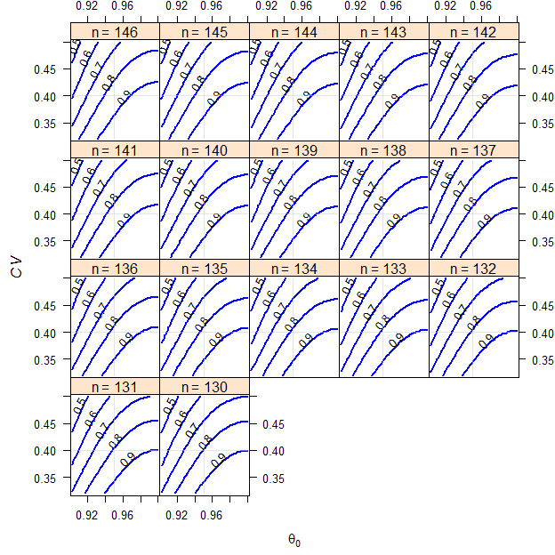
Fig. 1 Parallel design (T/R ratio 0.95, \(\small{CV}\) 0.40, dropout-rate 0.1).

Such patterns are typical for ABE.
We know already from the power analyis that the most sensitive parameter is \(\small{\theta_0}\), which can decrease from the assumed 0.95 to 0.9276 (maximum relative deviation –2.36%) until we reach a power of 0.70. The \(\small{CV}\) is much less sensitive, which can increase from the assumed 0.40 to 0.4552 (relative +13.8%). The least sensitive is the sample size itself. Hence, dropouts are in general of the least concern.

The lower right quadrants of each panel show ‘nice‘ combinations (\(\small{\theta_0}\) > assumed and \(\small{CV}\) < assumed). Higher power than targeted, great.
The other combinations are tricky. Since power is most sensitive to \(\small{\theta_0}\), it would need a substantially lower \(\small{CV}\) to compensate for a worse \(\small{\theta_0}\). Have a look at the 0.80 contour lines in the lower left quadrant of the first panel (no dropouts). If \(\small{\theta_0\approx 0.92}\) it would need \(\small{CV\approx 0.34}\) to preserve power. If the worst case hits and we have only 130 eligible subjects, it would need \(\small{CV\approx 0.32}\).
On the other hand, ‘better’ \(\small{\theta_0}\)s allow for higher \(\small{CV}\)s. That’s shown in the upper right quadrants. However, if the \(\small{CV}\) gets too large, even a \(\small{\theta_0}\) of 1 might not always give the target power.
In the upper left quadrants are the worst case combinations (\(\small{\theta_0}\) < assumed and _\(\small{CV}\) > assumed). It might still be possible to show BE though with a lower chance (power < target).

Since we assigned the result to an object x in the function call, we can explore what’s going on behind the curtain.

# assumed values
theta0  <- 0.95
CV      <- 0.40
target  <- 0.80
# vectors of values and extreme sample sizes
theta0s <- unique(x$theta0)
CVs     <- unique(x$CV)
n.range <- range(as.numeric(as.character(x$n)))
res     <- data.frame(scenario = c("closest",
                                   rep("worst", 2),
                                   rep("assumed", 2),
                                   rep("best", 2)),
                      theta0 = NA_real_, CV = NA_real_,
                      n = NA_integer_, power = NA_real_)
closest <- as.data.frame(x[which.min(abs(x$power - target)), ])
res[1, c(2:3, 5)] <- closest[c(1:2, 4)]
res[1, 4]         <- as.integer(as.character(closest$n))
worst             <- as.data.frame(x[x$theta0 == min(theta0s) &
                                     x$CV == max(CVs) &
                                   as.numeric(as.character(x$n)) %in% n.range, ])
res[2:3, c(2:3, 5)] <- worst[, c(1:2, 4)]
res[2:3, 4]         <- as.integer(as.character(worst$n))
assumed  <- as.data.frame(x[x$theta0 == theta0 & x$CV == CV &
                            as.numeric(as.character(x$n)) %in% n.range, ])
res[4:5, c(2:3, 5)] <- assumed[, c(1:2, 4)]
res[4:5, 4]         <- as.integer(as.character(assumed$n))
best    <- as.data.frame(x[x$theta0 == max(theta0s) &
                           x$CV == min(CVs) &
                           as.numeric(as.character(x$n)) %in% n.range, ])
res[6:7, c(2:3, 5)] <- best[, c(1:2, 4)]
res[6:7, 4]         <- as.integer(as.character(best$n))
res[, 2:5]          <- signif(res[, 2:5], 5)
print(res, row.names = FALSE)

#  scenario  theta0    CV   n   power
#   closest 0.99594 0.455 131 0.80004
#     worst 0.90250 0.500 146 0.44993
#     worst 0.90250 0.500 130 0.40992
#   assumed 0.95000 0.400 146 0.84606
#   assumed 0.95000 0.400 130 0.80351
#      best 1.00000 0.320 146 0.99201
#      best 1.00000 0.320 130 0.98395

closest shows the combination of \(\small{\theta_0}\), \(\small{CV}\), and \(\small{n}\) which is closest to the target power. Only for comparison. worst shows the combinations giving the lowest power for the large sample size (no dropouts) as well as for the planned sample size (anticipated dropout-rate realized). These are the values in the upper left corners of the first and last panels of the plot. Guess what assumed means… best shows the combinations giving the highest power. These are the values in the lower right corners of the first and last panels of the plot.

For real neRds only!

Power is a hypersurface depending on \(\small{\theta_0}\), \(\small{n}\), and \(\small{CV}\). Don’t try to imagine four-dimensional space – it may fry your brain! We can only show spatial projections at certain \(\small{CV\text{-}}\)values.

Fig. 2 Spatial projections of power for \(\small{\theta_0=0.80-1.00}\), \(\small{n=76-194}\), and \(\small{CV=0.30-0.50}\).

In the sensitivity analysis we ‘slice’ the hypersurface for a range of \(\small{\theta_0\textrm{-}}\) and \(\small{n\textrm{-}}\)values at certain \(\small{CV\textrm{s}}\). The magenta ribbon shows the \(\small{n=130-146}\) we planned for and the magenta line the \(\small{\theta_0=0.95}\) we assumed.

Inspecting the power-surfaces for a given \(\small{n}\), we see the maxima at \(\small{\theta_0=1}\) (\(\small{\log_{e}\theta_0=0}\)). Since power is symmetrical in \(\small{\log_{e}\textrm{-}}\)scale, we get identical ones for \(\small{\theta_0}\) and \(\small{1/\theta_0}\). That’s why here and in the script I don’t show \(\small{\theta_0>1}\). Furthermore, at the limits of the acceptance range (\(\small{\theta_1=0.80,\,\theta_2=1.25}\)) power \(\small{\leq 0.05}\), demonstrating that the Type I Error is controlled. For any given \(\small{\theta_0}\) power increases with \(\small{n}\) (asympotically approaching \(\small{1}\)).

The points show the \(\small{n}\) required to achieve our target power \(\small{\geq0.8}\) for \(\small{\theta_0=0.95}\). Note that with \(\small{CV=0.40}\) and \(\small{n=130}\) the line at \(\small{\theta_0=0.95}\) intersects the power-surface at \(\small{0.8035}\). We could have one more dropout than anticipated because with \(\small{n=129}\) we still achieve a power of \(\small{0.8005}\).

This explains also why with \(\small{CV>0.4283}\) it is futile to hope for power \(\small{\geq0.80}\) even if we face no dropouts (\(\small{n=146}\)). That’s also evident in the first panel of Fig. 1.

opt <- function(x) {
  # find maximum CV for target power
  # and given n, theta0, CV, design
  suppressMessages(
    power.TOST(CV = x, theta0 = theta0, design = design,
               n = res$n[i])) - target
}
theta0 <- 0.95
target <- 0.80
design <- "parallel"
CV     <- 0.40
n      <- 146:130L
txt    <- paste("power at least", sprintf("%.2f", target), "\n")
res    <- data.frame(n = n, do.rate = NA_real_, CV.max = NA_real_)
for (i in 1:nrow(res)) {
  res$CV.max[i] <- signif(uniroot(opt, interval = c(0.1, 2),
                                  extendInt = "yes",
                                  tol = 1e-8)$root, 4)
}
res$do.rate <- sprintf("%.4f", abs((res$n - max(n)) / max(n)))
cat(txt)
print(res, row.names = FALSE)

# power at least 0.80 
#    n do.rate CV.max
#  146  0.0000 0.4283
#  145  0.0068 0.4266
#  144  0.0137 0.4250
#  143  0.0205 0.4234
#  142  0.0274 0.4218
#  141  0.0342 0.4202
#  140  0.0411 0.4185
#  139  0.0479 0.4169
#  138  0.0548 0.4153
#  137  0.0616 0.4136
#  136  0.0685 0.4120
#  135  0.0753 0.4103
#  134  0.0822 0.4086
#  133  0.0890 0.4070
#  132  0.0959 0.4053
#  131  0.1027 0.4036
#  130  0.1096 0.4019

On the other hand, if \(\small{CV<0.40}\) we could achieve power \(\small{\geq0.90}\). Note the intersections of the \(\small{0.9\textrm{-}}\)line with \(\small{\theta_0=0.95}\) in Fig. 1.

opt <- function(x) {
  # find maximum CV for target power
  # and given n, theta0, CV, design
  suppressMessages(
    power.TOST(CV = x, theta0 = theta0, design = design,
               n = res$n[i])) - target
}
theta0 <- 0.95
target <- 0.90
design <- "parallel"
CV     <- 0.40
n      <- 146:130L
txt    <- paste("power at least", sprintf("%.2f", target), "\n")
res    <- data.frame(n = n, do.rate = NA_real_, CV.max = NA_real_)
for (i in 1:nrow(res)) {
  res$CV.max[i] <- signif(uniroot(opt, interval = c(0.1, 2),
                                  extendInt = "yes",
                                  tol = 1e-8)$root, 4)
}
res$do.rate <- sprintf("%.4f", abs((res$n - max(n)) / max(n)))
cat(txt)
print(res, row.names = FALSE)

# power at least 0.90 
#    n do.rate CV.max
#  146  0.0000 0.3635
#  145  0.0068 0.3622
#  144  0.0137 0.3608
#  143  0.0205 0.3595
#  142  0.0274 0.3581
#  141  0.0342 0.3568
#  140  0.0411 0.3554
#  139  0.0479 0.3541
#  138  0.0548 0.3527
#  137  0.0616 0.3513
#  136  0.0685 0.3500
#  135  0.0753 0.3486
#  134  0.0822 0.3472
#  133  0.0890 0.3458
#  132  0.0959 0.3444
#  131  0.1027 0.3430
#  130  0.1096 0.3416

In practice, anything \(\small{<0.7}\) should be avoided.

opt <- function(x) {
  # find maximum CV for target power
  # and given n, theta0, CV, design
  suppressMessages(
    power.TOST(CV = x, theta0 = theta0, design = design,
               n = res$n[i])) - target
}
theta0 <- 0.95
target <- 0.70
design <- "parallel"
CV     <- 0.40
n      <- 146:130L
txt    <- paste("power at least", sprintf("%.2f", target), "\n")
res    <- data.frame(n = n, do.rate = NA_real_, CV.max = NA_real_)
for (i in 1:nrow(res)) {
  res$CV.max[i] <- signif(uniroot(opt, interval = c(0.1, 2),
                                  extendInt = "yes",
                                  tol = 1e-8)$root, 4)
}
res$do.rate <- sprintf("%.4f", abs((res$n - max(n)) / max(n)))
cat(txt)
print(res, row.names = FALSE)

# power at least 0.70 
#    n do.rate CV.max
#  146  0.0000 0.4856
#  145  0.0068 0.4837
#  144  0.0137 0.4818
#  143  0.0205 0.4799
#  142  0.0274 0.4781
#  141  0.0342 0.4762
#  140  0.0411 0.4743
#  139  0.0479 0.4724
#  138  0.0548 0.4705
#  137  0.0616 0.4686
#  136  0.0685 0.4667
#  135  0.0753 0.4648
#  134  0.0822 0.4629
#  133  0.0890 0.4609
#  132  0.0959 0.4590
#  131  0.1027 0.4571
#  130  0.1096 0.4552

Consequently, \(\small{0.7}\) is the default minimum in the power analysis functions of PowerTOST (see this article).

Of course, power \(\small{\leq0.5}\) (the red lines in Fig. 2) doesn’t make sense. We could toss a coin as well…

Recall that we are assessing prospective (a priori, ante hoc) power. A study might still pass BE though with lower retrospective (a posteriori, post hoc) power. However, that’s not relevant for the decision (for details see this article).

top of section ↩︎ previous section ↩︎

Crossover Design

We assume a T/R-ratio (\(\small{\theta_0}\)) of 0.95, a \(\small{CV}\) of 0.25, target a power of 0.80 and anticipate a dropout-rate of 0.10 (10%).

# assign to an object
x <- sensitivity(CV = 0.25, theta0 = 0.95,
                 do.rate = 0.1, design = "2x2x2")

# Results for theta0 = 0.95 and CV = 0.25 
#   n   power do.rate
#  32 0.85726 0.00000
#  31 0.84584 0.03125
#  30 0.83425 0.06250
#  29 0.82093 0.09375
#  28 0.80744 0.12500

As shown in the corresponding articles about sample size estimation and power analyis, we need 28 subjects to achieve a power of 0.8074. We see that also in the last row of the output. In order to compensate for the dropout-rate we should dose 32 subjects in order to have 28 eligible subjects in the worst case. This is also seen in the first row of the output.

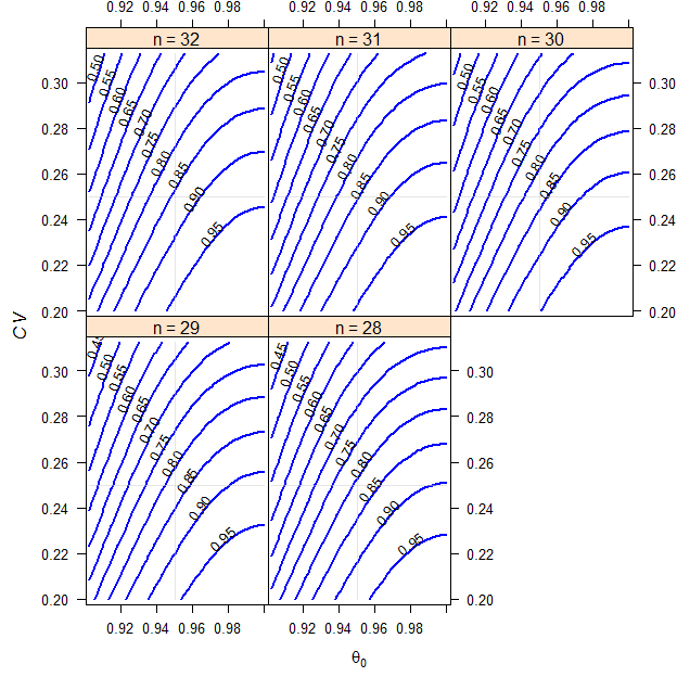
Fig. 3 Crossover design (T/R ratio 0.95, \(\small{CV}\) 0.25, dropout-rate 0.1).

# assumed values
theta0  <- 0.95
CV      <- 0.25
target  <- 0.80
# vectors of values and extreme sample sizes
theta0s <- unique(x$theta0)
CVs     <- unique(x$CV)
n.range <- range(as.numeric(as.character(x$n)))
res     <- data.frame(scenario = c("closest",
                                   rep("worst", 2),
                                   rep("assumed", 2),
                                   rep("best", 2)),
                      theta0 = NA_real_, CV = NA_real_,
                      n = NA_integer_, power = NA_real_)
closest <- as.data.frame(x[which.min(abs(x$power - target)), ])
res[1, c(2:3, 5)] <- closest[c(1:2, 4)]
res[1, 4]         <- as.integer(as.character(closest$n))
worst             <- as.data.frame(x[x$theta0 == min(theta0s) &
                                     x$CV == max(CVs) &
                                   as.numeric(as.character(x$n)) %in% n.range, ])
res[2:3, c(2:3, 5)] <- worst[, c(1:2, 4)]
res[2:3, 4]         <- as.integer(as.character(worst$n))
assumed  <- as.data.frame(x[x$theta0 == theta0 & x$CV == CV &
                            as.numeric(as.character(x$n)) %in% n.range, ])
res[4:5, c(2:3, 5)] <- assumed[, c(1:2, 4)]
res[4:5, 4]         <- as.integer(as.character(assumed$n))
best    <- as.data.frame(x[x$theta0 == max(theta0s) &
                           x$CV == min(CVs) &
                           as.numeric(as.character(x$n)) %in% n.range, ])
res[6:7, c(2:3, 5)] <- best[, c(1:2, 4)]
res[6:7, 4]         <- as.integer(as.character(best$n))
res[, 2:5]          <- signif(res[, 2:5], 5)
print(res, row.names = FALSE)

#  scenario  theta0      CV  n   power
#   closest 0.97156 0.28438 30 0.79980
#     worst 0.90250 0.31250 32 0.45406
#     worst 0.90250 0.31250 28 0.40602
#   assumed 0.95000 0.25000 32 0.85726
#   assumed 0.95000 0.25000 28 0.80744
#      best 1.00000 0.20000 32 0.99418
#      best 1.00000 0.20000 28 0.98603

top of section ↩︎ previous section ↩︎

C_max (Health Canada)

For Health Canada’s ABE only the point estimate of C_max has to lie with the conventional limits of 80.0–125.0%, i.e., the 90% confidence interval is not required like for all other agencies. In order to calculate power and estimate the sample size in the functions of PowerTOST we can use alpha = 0.5 in the calls.

We assume a T/R-ratio (\(\small{\theta_0}\)) of 0.90, a \(\small{CV}\) of 0.45, target a power of 0.80 and anticipate a dropout-rate of 0.10 (10%). We want to perform the study in a simple 2×2×2 crossover for Health Canada.

# assign to an object, no CI with alpha 0.5
x <- sensitivity(CV = 0.45, theta0 = 0.90,
                 do.rate = 0.1, design = "2x2x2",
                 alpha = 0.5)

# Results for theta0 = 0.9 and CV = 0.45 
#   n   power  do.rate
#  26 0.83575 0.000000
#  25 0.83028 0.038462
#  24 0.82496 0.076923
#  23 0.81885 0.115380
#  22 0.81292 0.153850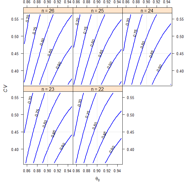

Fig. 4 Crossover design (T/R ratio 0.90, \(\small{CV}\) 0.45, dropout-rate 0.1).
Assessing the point estimate of C_max for Health Canada.

Only in very rare cases (if the CV of AUC is substantially smaller than the one of C_max) you will have to base the sample size on C_max.

# assumed values
theta0  <- 0.90
CV      <- 0.45
target  <- 0.80
# vectors of values and extreme sample sizes
theta0s <- unique(x$theta0)
CVs     <- unique(x$CV)
n.range <- range(as.numeric(as.character(x$n)))
res     <- data.frame(scenario = c("closest",
                                   rep("worst", 2),
                                   rep("assumed", 2),
                                   rep("best", 2)),
                      theta0 = NA_real_, CV = NA_real_,
                      n = NA_integer_, power = NA_real_)
closest <- as.data.frame(x[which.min(abs(x$power - target)), ])
res[1, c(2:3, 5)] <- closest[c(1:2, 4)]
res[1, 4]         <- as.integer(as.character(closest$n))
worst             <- as.data.frame(x[x$theta0 == min(theta0s) &
                                     x$CV == max(CVs) &
                                   as.numeric(as.character(x$n)) %in% n.range, ])
res[2:3, c(2:3, 5)] <- worst[, c(1:2, 4)]
res[2:3, 4]         <- as.integer(as.character(worst$n))
assumed  <- as.data.frame(x[x$theta0 == theta0 & x$CV == CV &
                            as.numeric(as.character(x$n)) %in% n.range, ])
res[4:5, c(2:3, 5)] <- assumed[, c(1:2, 4)]
res[4:5, 4]         <- as.integer(as.character(assumed$n))
best    <- as.data.frame(x[x$theta0 == max(theta0s) &
                           x$CV == min(CVs) &
                           as.numeric(as.character(x$n)) %in% n.range, ])
res[6:7, c(2:3, 5)] <- best[, c(1:2, 4)]
res[6:7, 4]         <- as.integer(as.character(best$n))
res[, 2:5]          <- signif(res[, 2:5], 5)
print(res, row.names = FALSE)

#  scenario  theta0      CV  n   power
#   closest 0.87424 0.39375 26 0.80000
#     worst 0.85500 0.56250 26 0.67174
#     worst 0.85500 0.56250 22 0.65483
#   assumed 0.90000 0.45000 26 0.83575
#   assumed 0.90000 0.45000 22 0.81292
#      best 0.94737 0.36000 26 0.95752
#      best 0.94737 0.36000 22 0.94168

top of section ↩︎ previous section ↩︎

ABEL (EMA, …)

This is the method recommended by agencies accepting SABE – except the FDA and China’s CDE (both recommend RSABE instead).

We assume a T/R-ratio (\(\small{\theta_0}\)) of 0.90, a \(\small{CV}\) of 0.45, target a power of 0.80 and anticipate a dropout-rate of 0.15 (15%). We want to perform the study in a 2-sequence 4-period full replicate study (TRTR|RTRT, TRRT|RTTR or TTRR|RRTT).
Note that this is time-consuming because for every of the 4,732 combinations 10⁵ simulations are performed. That’s a lot.

# assign to an object
# normally don't turn off the progress bar
x <- sensitivity(CV = 0.45, theta0 = 0.90,
                 do.rate = 0.15, design = "2x2x4",
                 SABE = TRUE, regulator = "EMA",
                 info = FALSE, progress = FALSE)

# Results for theta0 = 0.9 and CV = 0.45 
#   n   power  do.rate
#  34 0.87196 0.000000
#  33 0.86302 0.029412
#  32 0.85528 0.058824
#  31 0.84556 0.088235
#  30 0.83397 0.117650
#  29 0.82366 0.147060
#  28 0.81116 0.176470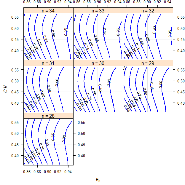

Fig. 5 2×2×4 replicate design (T/R ratio 0.90, \(\small{CV}\) 0.45, dropout-rate 0.15).
ABEL intended for the EMA.

Such a pattern is typical for all variants of SABE. The idea of reference-scaling is to maintain power irrespective of the \(\small{CV}\). Therefore, the \(\small{CV}\) is the least sensitive parameter – it can increase from the assumed 0.45 to 0.6629 (relative +47.3%) until power will be only 0.70. On the other hand, if the \(\small{CV}\) decreases, power decreases as well because we can expand the limits less. However, like in ABE the most sensitive parameter is \(\small{\theta_0}\) and the least sensitive is the sample size itself.

# assumed values
theta0  <- 0.90
CV      <- 0.45
target  <- 0.80
# vectors of values and extreme sample sizes
theta0s <- unique(x$theta0)
CVs     <- unique(x$CV)
n.range <- range(as.numeric(as.character(x$n)))
res     <- data.frame(scenario = c("closest",
                                   rep("worst", 2),
                                   rep("assumed", 2),
                                   rep("best", 2)),
                      theta0 = NA_real_, CV = NA_real_,
                      n = NA_integer_, power = NA_real_)
closest <- as.data.frame(x[which.min(abs(x$power - target)), ])
res[1, c(2:3, 5)] <- closest[c(1:2, 4)]
res[1, 4]         <- as.integer(as.character(closest$n))
worst             <- as.data.frame(x[x$theta0 == min(theta0s) &
                                     x$CV == max(CVs) &
                                   as.numeric(as.character(x$n)) %in% n.range, ])
res[2:3, c(2:3, 5)] <- worst[, c(1:2, 4)]
res[2:3, 4]         <- as.integer(as.character(worst$n))
assumed  <- as.data.frame(x[x$theta0 == theta0 & x$CV == CV &
                            as.numeric(as.character(x$n)) %in% n.range, ])
res[4:5, c(2:3, 5)] <- assumed[, c(1:2, 4)]
res[4:5, 4]         <- as.integer(as.character(assumed$n))
best    <- as.data.frame(x[x$theta0 == max(theta0s) &
                           x$CV == min(CVs) &
                           as.numeric(as.character(x$n)) %in% n.range, ])
res[6:7, c(2:3, 5)] <- best[, c(1:2, 4)]
res[6:7, 4]         <- as.integer(as.character(best$n))
res[, 2:5]          <- signif(res[, 2:5], 5)
print(res, row.names = FALSE)

#  scenario  theta0      CV  n   power
#   closest 0.89734 0.44438 28 0.80002
#     worst 0.85500 0.56250 34 0.69661
#     worst 0.85500 0.56250 28 0.61691
#   assumed 0.90000 0.45000 34 0.87196
#   assumed 0.90000 0.45000 28 0.81116
#      best 0.94737 0.36000 34 0.95507
#      best 0.94737 0.36000 28 0.91921

top of section ↩︎ previous section ↩︎

ABEL (Health Canada)

Similar to above but the upper cap of scaling is \(\small{CV_\textrm{wR}\sim 57.4\%}\) instead of \(\small{CV_\textrm{wR}=50\%}\).

We assume a T/R-ratio (\(\small{\theta_0}\)) of 0.90, a \(\small{CV}\) of 0.50, target a power of 0.80 and anticipate a dropout-rate of 0.15 (15%). We want to perform the study in a 2-sequence 4-period full replicate study (TRTR|RTRT, TRRT|RTTR or TTRR|RRTT).

# assign to an object; normally show the information
# and don't turn off the progress bar
x <- sensitivity(CV = 0.50, theta0 = 0.90,
                 do.rate = 0.15, design = "2x2x4",
                 SABE = TRUE, regulator = "HC",
                 info = FALSE, progress = FALSE)

# Results for theta0 = 0.9 and CV = 0.5 
#   n   power  do.rate
#  34 0.87012 0.000000
#  33 0.86191 0.029412
#  32 0.85446 0.058824
#  31 0.84307 0.088235
#  30 0.83417 0.117650
#  29 0.82398 0.147060
#  28 0.81266 0.176470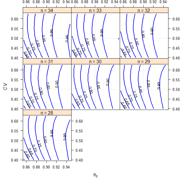

Fig. 6 2×2×4 replicate design (T/R ratio 0.90, \(\small{CV}\) 0.50, dropout-rate 0.15).
ABEL intended for Health Canada.

The pattern is similar to the previous example for the EMA but more relaxed due to the higher cap of scaling.

# assumed values
theta0  <- 0.90
CV      <- 0.50
target  <- 0.80
# vectors of values and extreme sample sizes
theta0s <- unique(x$theta0)
CVs     <- unique(x$CV)
n.range <- range(as.numeric(as.character(x$n)))
res     <- data.frame(scenario = c("closest",
                                   rep("worst", 2),
                                   rep("assumed", 2),
                                   rep("best", 2)),
                      theta0 = NA_real_, CV = NA_real_,
                      n = NA_integer_, power = NA_real_)
closest <- as.data.frame(x[which.min(abs(x$power - target)), ])
res[1, c(2:3, 5)] <- closest[c(1:2, 4)]
res[1, 4]         <- as.integer(as.character(closest$n))
worst             <- as.data.frame(x[x$theta0 == min(theta0s) &
                                     x$CV == max(CVs) &
                                   as.numeric(as.character(x$n)) %in% n.range, ])
res[2:3, c(2:3, 5)] <- worst[, c(1:2, 4)]
res[2:3, 4]         <- as.integer(as.character(worst$n))
assumed  <- as.data.frame(x[x$theta0 == theta0 & x$CV == CV &
                            as.numeric(as.character(x$n)) %in% n.range, ])
res[4:5, c(2:3, 5)] <- assumed[, c(1:2, 4)]
res[4:5, 4]         <- as.integer(as.character(assumed$n))
best    <- as.data.frame(x[x$theta0 == max(theta0s) &
                           x$CV == min(CVs) &
                           as.numeric(as.character(x$n)) %in% n.range, ])
res[6:7, c(2:3, 5)] <- best[, c(1:2, 4)]
res[6:7, 4]         <- as.integer(as.character(best$n))
res[, 2:5]          <- signif(res[, 2:5], 5)
print(res, row.names = FALSE)

#  scenario  theta0      CV  n   power
#   closest 0.88194 0.60625 32 0.80004
#     worst 0.85500 0.62500 34 0.71794
#     worst 0.85500 0.62500 28 0.65997
#   assumed 0.90000 0.50000 34 0.87012
#   assumed 0.90000 0.50000 28 0.81266
#      best 0.94737 0.40000 34 0.94997
#      best 0.94737 0.40000 28 0.90649

top of section ↩︎ previous section ↩︎

GCC

# assign to an object; normally show the information
# and don't turn off the progress bar
# set special limits of the CV to show the switching
# at 30%
x <- sensitivity(CV = 0.45, theta0 = 0.90,
                 do.rate = 0.15, design = "2x2x4",
                 CV.lo = 0.25, CV.hi = 0.50,
                 SABE = TRUE, regulator = "GCC",
                 info = FALSE, progress = FALSE)

# Results for theta0 = 0.9 and CV = 0.45 
#   n   power  do.rate
#  44 0.87568 0.000000
#  43 0.86886 0.022727
#  42 0.86190 0.045455
#  41 0.85396 0.068182
#  40 0.84624 0.090909
#  39 0.83802 0.113640
#  38 0.82943 0.136360
#  37 0.82049 0.159090
#  36 0.81116 0.181820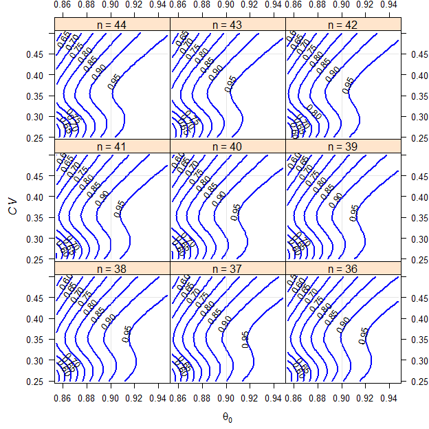

Fig. 7 2×2×4 replicate design (T/R ratio 0.90, \(\small{CV}\) 0.45, dropout-rate 0.15).
ABE with Widened Limits intended for the GCC.

That’s a special case because for \(\small{CV_\textrm{wR}\leq30\%}\) the conventional limits of 80.00–125.00% have to be applied and for \(\small{CV_\textrm{wR}>30\%}\) the limits are directly widened to 75.00–133.33%. Furthermore, there is no upper cap of scaling like in ABEL.

# assumed values
theta0  <- 0.90
CV      <- 0.45
target  <- 0.80
# vectors of values and extreme sample sizes
theta0s <- unique(x$theta0)
CVs     <- unique(x$CV)
n.range <- range(as.numeric(as.character(x$n)))
res     <- data.frame(scenario = c("closest",
                                   rep("worst", 2),
                                   rep("assumed", 2),
                                   rep("best", 2)),
                      theta0 = NA_real_, CV = NA_real_,
                      n = NA_integer_, power = NA_real_)
closest <- as.data.frame(x[which.min(abs(x$power - target)), ])
res[1, c(2:3, 5)] <- closest[c(1:2, 4)]
res[1, 4]         <- as.integer(as.character(closest$n))
worst             <- as.data.frame(x[x$theta0 == min(theta0s) &
                                     x$CV == max(CVs) &
                                   as.numeric(as.character(x$n)) %in% n.range, ])
res[2:3, c(2:3, 5)] <- worst[, c(1:2, 4)]
res[2:3, 4]         <- as.integer(as.character(worst$n))
assumed  <- as.data.frame(x[x$theta0 == theta0 & x$CV == CV &
                            as.numeric(as.character(x$n)) %in% n.range, ])
res[4:5, c(2:3, 5)] <- assumed[, c(1:2, 4)]
res[4:5, 4]         <- as.integer(as.character(assumed$n))
best    <- as.data.frame(x[x$theta0 == max(theta0s) &
                           x$CV == min(CVs) &
                           as.numeric(as.character(x$n)) %in% n.range, ])
res[6:7, c(2:3, 5)] <- best[, c(1:2, 4)]
res[6:7, 4]         <- as.integer(as.character(best$n))
res[, 2:5]          <- signif(res[, 2:5], 5)
print(res, row.names = FALSE)

#  scenario  theta0      CV  n   power
#   closest 0.87039 0.39583 42 0.80000
#     worst 0.85500 0.50000 44 0.57507
#     worst 0.85500 0.50000 36 0.50533
#   assumed 0.90000 0.45000 44 0.87568
#   assumed 0.90000 0.45000 36 0.81116
#      best 0.94737 0.25000 44 0.99860
#      best 0.94737 0.25000 36 0.99354

top of section ↩︎ previous section ↩︎

RSABE

This is the SABE-method recommended by the FDA and China’s CDE.

# assign to an object; normally show the information
# and don't turn off the progress bar
x <- sensitivity(CV = 0.45, theta0 = 0.90,
                 do.rate = 0.15, design = "2x2x4",
                 SABE = TRUE, regulator = "FDA",
                 info = FALSE, progress = FALSE)

# Results for theta0 = 0.9 and CV = 0.45 
#   n   power  do.rate
#  30 0.88991 0.000000
#  29 0.88095 0.033333
#  28 0.87287 0.066667
#  27 0.86119 0.100000
#  26 0.85083 0.133330
#  25 0.83767 0.166670
#  24 0.82450 0.200000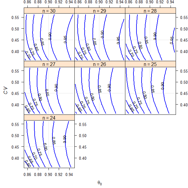

Fig. 8 2×2×4 replicate design (T/R ratio 0.90, \(\small{CV}\) 0.45, dropout-rate 0.15).
RSABE intended for the FDA.

Contrary to the variants of ABEL, there is no upper cap of scaling. Together with the more steep scaling (regulatory constant \(\small{\theta_\textrm{s}\sim 0.893}\) instead of \(\small{k=0.760}\) for the EMA and Health Canada) sample sizes are always smaller than for these agencies. Or the way ’round, for a given sample size the method is more permissive. For details see another article.

# assumed values
theta0  <- 0.90
CV      <- 0.45
target  <- 0.80
# vectors of values and extreme sample sizes
theta0s <- unique(x$theta0)
CVs     <- unique(x$CV)
n.range <- range(as.numeric(as.character(x$n)))
res     <- data.frame(scenario = c("closest",
                                   rep("worst", 2),
                                   rep("assumed", 2),
                                   rep("best", 2)),
                      theta0 = NA_real_, CV = NA_real_,
                      n = NA_integer_, power = NA_real_)
closest <- as.data.frame(x[which.min(abs(x$power - target)), ])
res[1, c(2:3, 5)] <- closest[c(1:2, 4)]
res[1, 4]         <- as.integer(as.character(closest$n))
worst             <- as.data.frame(x[x$theta0 == min(theta0s) &
                                     x$CV == max(CVs) &
                                   as.numeric(as.character(x$n)) %in% n.range, ])
res[2:3, c(2:3, 5)] <- worst[, c(1:2, 4)]
res[2:3, 4]         <- as.integer(as.character(worst$n))
assumed  <- as.data.frame(x[x$theta0 == theta0 & x$CV == CV &
                            as.numeric(as.character(x$n)) %in% n.range, ])
res[4:5, c(2:3, 5)] <- assumed[, c(1:2, 4)]
res[4:5, 4]         <- as.integer(as.character(assumed$n))
best    <- as.data.frame(x[x$theta0 == max(theta0s) &
                           x$CV == min(CVs) &
                           as.numeric(as.character(x$n)) %in% n.range, ])
res[6:7, c(2:3, 5)] <- best[, c(1:2, 4)]
res[6:7, 4]         <- as.integer(as.character(best$n))
res[, 2:5]          <- signif(res[, 2:5], 5)
print(res, row.names = FALSE)

#  scenario  theta0      CV  n   power
#   closest 0.88579 0.55406 25 0.79998
#     worst 0.85500 0.56250 30 0.73713
#     worst 0.85500 0.56250 24 0.68706
#   assumed 0.90000 0.45000 30 0.88991
#   assumed 0.90000 0.45000 24 0.82450
#      best 0.94737 0.36000 30 0.95638
#      best 0.94737 0.36000 24 0.90998

top of section ↩︎ previous section ↩︎

NTIDs (FDA, CDE)

We assume a T/R-ratio (\(\small{\theta_0}\)) of 0.975, a \(\small{CV}\) of 0.125, target a power of 0.80 and anticipate a dropout-rate of 0.15 (15%). We want to perform the study in a 2-sequence 4-period full replicate study (TRTR|RTRT, TRRT|RTTR or TTRR|RRTT) according to the rules of the FDA.⁷

# assign to an object; normally show the information
# and don't turn off the progress bar
# custom settings of the axes
x <- sensitivity(CV = 0.125, theta0 = 0.975, do.rate = 0.15,
                 SABE = TRUE, regulator = "FDA", ntid = TRUE,
                 design = "2x2x4", CV.hi = 0.3, theta0.hi = 1,
                 info = FALSE, progress = FALSE)

# Results for theta0 = 0.975 and CV = 0.125 
#   n   power do.rate
#  20 0.90910    0.00
#  19 0.89039    0.05
#  18 0.87340    0.10
#  17 0.84853    0.15
#  16 0.82278    0.20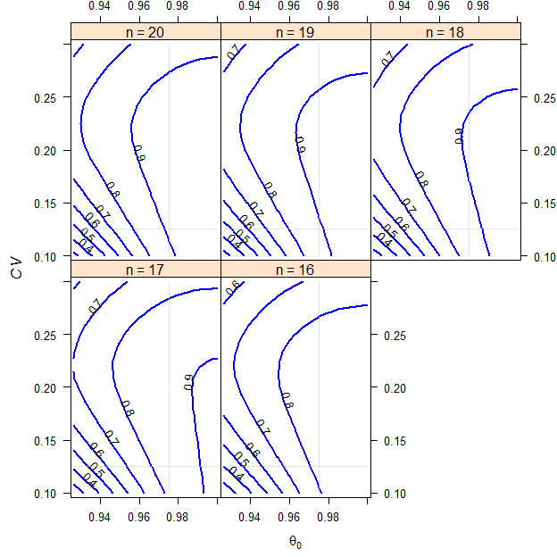

Fig. 9 2×2×4 replicate design (T/R ratio 0.975, \(\small{CV}\) 0.125, dropout-rate 0.15).
RSABE for NTIDs.

Here we see a pattern different to all other appoaches. Since there is an implied upper cap of scaling at \(\small{CV \approx 21.4188\%}\) (when the conventional limits of 80.00–125.00% have to be used), for any given \(\small{\theta_0}\) and a larger \(\small{CV}\), power curves ‘bend’ sharply to the right. In other words, we will loose power fast. With a smaller \(\small{CV}\) we will also loose power because the implied limits get narrower.

# assumed values
theta0  <- 0.975
CV      <- 0.125
target  <- 0.80
# vectors of values and extreme sample sizes
theta0s <- unique(x$theta0)
CVs     <- unique(x$CV)
n.range <- range(as.numeric(as.character(x$n)))
res     <- data.frame(scenario = c("closest",
                                   rep("worst", 2),
                                   rep("assumed", 2),
                                   rep("best", 2)),
                      theta0 = NA_real_, CV = NA_real_,
                      n = NA_integer_, power = NA_real_)
closest <- as.data.frame(x[which.min(abs(x$power - target)), ])
res[1, c(2:3, 5)] <- closest[c(1:2, 4)]
res[1, 4]         <- as.integer(as.character(closest$n))
worst             <- as.data.frame(x[x$theta0 == min(theta0s) &
                                     x$CV == max(CVs) &
                                   as.numeric(as.character(x$n)) %in% n.range, ])
res[2:3, c(2:3, 5)] <- worst[, c(1:2, 4)]
res[2:3, 4]         <- as.integer(as.character(worst$n))
assumed  <- as.data.frame(x[x$theta0 == theta0 & x$CV == CV &
                            as.numeric(as.character(x$n)) %in% n.range, ])
res[4:5, c(2:3, 5)] <- assumed[, c(1:2, 4)]
res[4:5, 4]         <- as.integer(as.character(assumed$n))
best    <- as.data.frame(x[x$theta0 == max(theta0s) &
                           x$CV == min(CVs) &
                           as.numeric(as.character(x$n)) %in% n.range, ])
res[6:7, c(2:3, 5)] <- best[, c(1:2, 4)]
res[6:7, 4]         <- as.integer(as.character(best$n))
res[, 2:5]          <- signif(res[, 2:5], 5)
print(res, row.names = FALSE)

#  scenario  theta0      CV  n   power
#   closest 0.95083 0.26667 18 0.79998
#     worst 0.92625 0.30000 18 0.61867
#     worst 0.92625 0.30000 16 0.55245
#   assumed 0.97500 0.12500 18 0.87340
#   assumed 0.97500 0.12500 16 0.82278
#      best 1.00000 0.10000 18 0.92770
#      best 1.00000 0.10000 16 0.88336

top of section ↩︎ previous section ↩︎

NTIDs (others)

Only the FDA and China’s CDE recommend RSABE. All other agencies recommend conventional ABE with limits fixed at 90.00–111.11% (though not necessarily for all PK metrics).

# assign to an object; custom settings of the axes
x <- sensitivity(CV = 0.125, theta0 = 0.975, do.rate = 0.15,
                 theta1 = 0.90, design = "2x2x4", CV.hi = 0.3,
                 theta0.hi = 1, info = FALSE)

# Results for theta0 = 0.975 and CV = 0.125 
#   n   power do.rate
#  20 0.88256    0.00
#  19 0.86597    0.05
#  18 0.84903    0.10
#  17 0.82762    0.15
#  16 0.80592    0.20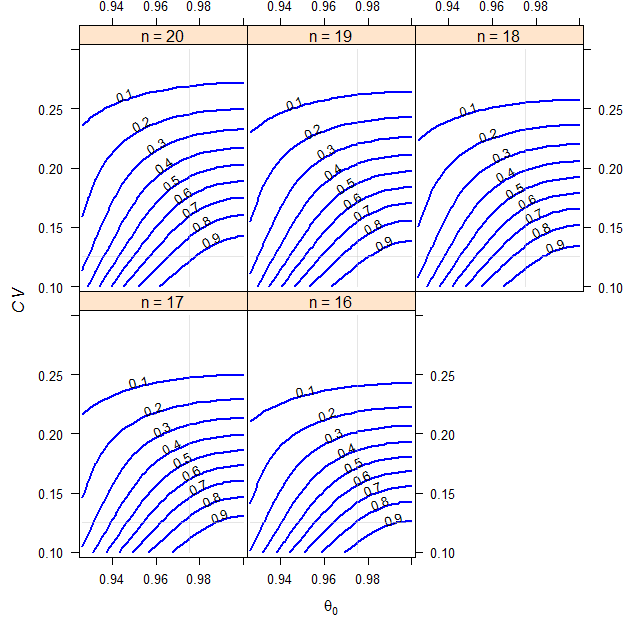

Fig. 10 2×2×4 replicate design (T/R ratio 0.975, \(\small{CV}\) 0.125, dropout-rate 0.15).
ABE with fixed narrower limits.

If the \(\small{CV}\) gets larger, we will quickly loose power and it will be practically impossible to show BE. Contrary to the reference-scaled approach, with smaller \(\small{CV\textrm{s}}\) we will gain power.

# assumed values
theta0  <- 0.975
CV      <- 0.125
target  <- 0.80
# vectors of values and extreme sample sizes
theta0s <- unique(x$theta0)
CVs     <- unique(x$CV)
n.range <- range(as.numeric(as.character(x$n)))
res     <- data.frame(scenario = c("closest",
                                   rep("worst", 2),
                                   rep("assumed", 2),
                                   rep("best", 2)),
                      theta0 = NA_real_, CV = NA_real_,
                      n = NA_integer_, power = NA_real_)
closest <- as.data.frame(x[which.min(abs(x$power - target)), ])
res[1, c(2:3, 5)] <- closest[c(1:2, 4)]
res[1, 4]         <- as.integer(as.character(closest$n))
worst             <- as.data.frame(x[x$theta0 == min(theta0s) &
                                     x$CV == max(CVs) &
                                   as.numeric(as.character(x$n)) %in% n.range, ])
res[2:3, c(2:3, 5)] <- worst[, c(1:2, 4)]
res[2:3, 4]         <- as.integer(as.character(worst$n))
assumed  <- as.data.frame(x[x$theta0 == theta0 & x$CV == CV &
                            as.numeric(as.character(x$n)) %in% n.range, ])
res[4:5, c(2:3, 5)] <- assumed[, c(1:2, 4)]
res[4:5, 4]         <- as.integer(as.character(assumed$n))
best    <- as.data.frame(x[x$theta0 == max(theta0s) &
                           x$CV == min(CVs) &
                           as.numeric(as.character(x$n)) %in% n.range, ])
res[6:7, c(2:3, 5)] <- best[, c(1:2, 4)]
res[6:7, 4]         <- as.integer(as.character(best$n))
res[, 2:5]          <- signif(res[, 2:5], 5)
print(res, row.names = FALSE)

#  scenario  theta0      CV  n   power
#   closest 0.95083 0.28333 17 0.80017
#     worst 0.92625 0.30000 18 0.66721
#     worst 0.92625 0.30000 16 0.61711
#   assumed 0.97500 0.12500 18 1.00000
#   assumed 0.97500 0.12500 16 1.00000
#      best 1.00000 0.10000 18 1.00000
#      best 1.00000 0.10000 16 1.00000

top of section ↩︎ previous section ↩︎

Final Remark

Assuming that values from the literature – and from a pilot study as well – are the true ones, would be a serious flaw. That’s the ‘Carved-in-Stone’ approach, which is discussed in the other articles about sample size estimation.

Even more so, you should not believe⁸ that the assumed values will be exactly realized in the study.

The sensitivity analysis can give you an idea what might happen and protects you against surprises.

previous section ↩︎

Postscript

Note that power curves for ABE are concave – running from the lower left to the upper right. Ideally in SABE power would be independent from \(\small{CV}\) and therefore, straight vertical lines. Due to the transition from ABE to SABE at \(\small{CV=30\%}\), the point estimate constraint of 80.00–125.00%, and – in ABEL – the upper cap of scaling (EMA \(\small{CV=50\%}\), Health Canada \(\small{CV \sim 57.4\%}\)), they aren’t.

You could misuse the script to produce results similar to Tóthfalusi and Endrényi⁹ (below an example for the EMA’s ABEL in a partial replicate design, i.e., TRR|RTR|RRT). Note that the authors reported a sample size of 44 in Table A1, which is likely due to their lower number of simulations (10,000 instead of 10⁵ in PowerTOST). For details see the case study in the article about simulations.

# dropout-rate zero gives only the estimated sample size
# specified limits of theta0 and CV, higher resolution
# smaller size of plot, draw point at theta0 / CV
x <- sensitivity(CV = 0.40, theta0 = 0.90,
                 do.rate = 0, design = "2x3x3",
                 theta0.lo = 0.80, theta0.hi = 1.25,
                 CV.lo = 0.30, CV.hi = 0.80,
                 SABE = TRUE, regulator = "EMA",
                 mesh = 50, contours = 20,
                 width = 5.5, height = 5.5,
                 point = TRUE, info = FALSE,
                 progress = FALSE)

# Results for theta0 = 0.9 and CV = 0.4 
#   n   power do.rate
#  42 0.80059       0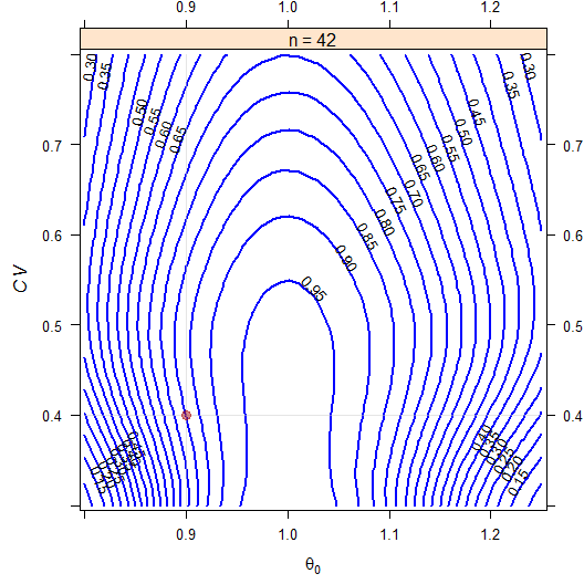

Fig. 11 2×3×3 partial replicate design (T/R ratio 0.90, \(\small{CV}\) 0.40, no dropouts).
ABEL intended for the EMA.

Heteroscedasticity

For neRs only.

As mentioned in the beginning, so far we considered only strict homoscedasticity. However, variances of products must not neccessarily be equal. Since biopharmaceutical technology improves, regularly \(\small{s_\textrm{wT}^2<{s_\textrm{wR}^2}}\). If this is the case, we get an incentive on the sample size: Scaling depends on \(\small{s_\textrm{wR}}\), whereas the confidence interval on the pooled \(\small{s_\textrm{w}}\).

Furthermore, a comparison of the \(\small{s_\textrm{wT}/{s_\textrm{wR}}}\)-ratio is part of the FDA’s and China’s CDE approaches for NTIDs and HVNTIDs. In both a full replicate design is mandatory.
In the former not only passing RSABE is required but also passing ABE and \(\small{s_\textrm{wT}/{s_\textrm{wR}}\leq2.5}\).
In the latter passing ABE is required and \(\small{s_\textrm{wT}/{s_\textrm{wR}}\leq 2.5}\).

This complicates things a lot. I’m afraid that there is no convenient way out. We can only estimate the sample size for assumed CV-combinations and assess various T/R-ratios for their impact on power.

power.hetero <- function(CV, theta0s, method, regulator, ...) {
  if (!method %in% c("ABEL", "RSABE", "NTID", "HVNTID"))
    stop("method must be \"ABEL\", \"RSABE\", ",
         "\"NTID\", or \"HVNTID\".")
  if (length(CV) == 1) CV[2] <- CV # homoscedastic
  res <- data.frame(n = n, CV.T = CV[1], CV.R = CV[2],
                    theta0 = theta0s, power = NA_real_)
  if (method == "ABEL") {
    if (!regulator %in% c("EMA", "HC", "GCC"))
      stop("regulator must be \"EMA\", \"HC\", or \"GCC\".")
    for (i in seq_along(theta0s)) {
      res$power[i] <- suppressMessages(
                        power.scABEL(CV = CV, theta0 = theta0s[i], ...))
    }
  }
  if (method == "RSABE") {
    if (!regulator == "FDA")
      stop("regulator must be \"FDA\".")
    if (!design %in% c("2x2x3", "2x2x4", "2x3x3"))
      stop("design must be \"2x2x3\", \"2x2x4\", or \"2x3x3\".")
    for (i in seq_along(theta0s)) {
      res$power[i] <- suppressMessages(
                        power.RSABE(CV = CV, theta0 = theta0s[i], ...))
    }
  }
  if (method == "NTID") {
    if (!design %in% c("2x2x4", "2x2x3"))
      stop("design must be \"2x2x4\", \"2x2x3\".")
    res <- cbind(res, p.SABE = NA_real_, p.ABE = NA_real_,
                 p.sratio = NA_real_)
    for (i in seq_along(theta0s)) {
      res[i, 5:8] <- suppressMessages(
                       power.NTID(CV = CV, theta0 = theta0s[i],
                                  details = TRUE, ...))
    }
  }
  if (method == "HVNTID") {
    if (!design %in% c("2x2x4", "2x2x3"))
      stop("design must be \"2x2x4\", \"2x2x3\".")
    res <- cbind(res, p.ABE = NA_real_, p.sratio = NA_real_)
    for (i in seq_along(theta0s)) {
      res[i, 5:7] <- suppressMessages(
                       power.HVNTID(CV = CV, theta0 = theta0s[i],
                                    details = TRUE, ...))
    }
  }
  return(res)
}

ABEL (EMA)

Let’s assume that \(\small{CV_\textrm{wT} = 0.414}\) and \(\small{CV_\textrm{wR} = 0.484}\), i.e, \(\small{s_\textrm{wT}^2/s_\textrm{wR}^2=0.75}\). Note that \(\small{CV_\textrm{w} = 0.45}\) like in the homoscedastic example above.

theta0  <- 0.90
CV      <- signif(CVp2CV(CV = 0.45, ratio = 0.75), 3) # T and R
design  <- "2x2x4"
theta0s <- seq(0.85, 1, 0.025)
n       <- sampleN.scABEL(CV = CV, theta0 = theta0, design = design,
                          details = FALSE, print = FALSE)[["Sample size"]]
x       <- power.hetero(CV = CV, theta0s = theta0s, method = "ABEL",
                        regulator = "EMA", n = n, design = design)
print(x, row.names = FALSE)

#   n  CV.T  CV.R theta0   power
#  24 0.414 0.484  0.850 0.59776
#  24 0.414 0.484  0.875 0.70912
#  24 0.414 0.484  0.900 0.80193
#  24 0.414 0.484  0.925 0.87140
#  24 0.414 0.484  0.950 0.91738
#  24 0.414 0.484  0.975 0.94320
#  24 0.414 0.484  1.000 0.95187

We need four fewer subjects than for \(\small{CV_\textrm{wT}=CV_\textrm{wR}=0.45}\) because the expanded limits for \(\small{CV_\textrm{wR} = 0.484}\) are with 70.56–141.72% more relaxed than the 72.15–138.59% for \(\small{CV_\textrm{wR}=0.45}\).

RSABE (FDA)

theta0  <- 0.90
CV      <- signif(CVp2CV(CV = 0.45, ratio = 0.75), 3) # T and R
design  <- "2x2x4"
theta0s <- seq(0.85, 1, 0.025)
n       <- sampleN.RSABE(CV = CV, theta0 = theta0, design = design,
                         details = FALSE, print = FALSE)[["Sample size"]]
x       <- power.hetero(CV = CV, theta0s = theta0s, method = "RSABE",
                        regulator = "FDA", n = n, design = design)
print(x, row.names = FALSE)

#   n  CV.T  CV.R theta0   power
#  20 0.414 0.484  0.850 0.62417
#  20 0.414 0.484  0.875 0.72109
#  20 0.414 0.484  0.900 0.80146
#  20 0.414 0.484  0.925 0.86057
#  20 0.414 0.484  0.950 0.90121
#  20 0.414 0.484  0.975 0.92427
#  20 0.414 0.484  1.000 0.93294

We need four fewer subjects than for \(\small{CV_\textrm{wT}=CV_\textrm{wR}=0.45}\).

NTID (FDA, CDE)

Let’s assume that \(\small{CV_\textrm{wT} = 0.116}\) and \(\small{CV_\textrm{wR} = 0.134}\), i.e, \(\small{s_\textrm{wT}^2/s_\textrm{wR}^2=0.75}\). Note that \(\small{CV_\textrm{w} = 0.125}\) like in the homoscedastic example above.

theta0  <- 0.975
CV      <- signif(CVp2CV(CV = 0.125, ratio = 0.75), 3) # T and R
design  <- "2x2x4"
theta0s <- seq(0.9, 1, 0.025)
n       <- sampleN.NTID(CV = CV, theta0 = theta0, design = design,
                        details = FALSE, print = FALSE)[["Sample size"]]
x       <- power.hetero(CV = CV, theta0s = theta0s, method = "NTID",
                        regulator = "FDA", n = n, design = design)
print(x, row.names = FALSE)

#   n  CV.T  CV.R theta0   power  p.SABE   p.ABE p.sratio
#  14 0.116 0.134  0.900 0.20478 0.20510 0.95292  0.96889
#  14 0.116 0.134  0.925 0.42218 0.42456 0.99270  0.96889
#  14 0.116 0.134  0.950 0.65763 0.66532 0.99935  0.96889
#  14 0.116 0.134  0.975 0.82384 0.83715 0.99997  0.96889
#  14 0.116 0.134  1.000 0.88029 0.89607 1.00000  0.96889

Note that the output contains not only the overall power but also the probability to pass SABE, ABE, and the \(\small{s_\textrm{wT}/{s_\textrm{wR}}\text{-}}\)test.
We need two fewer subjects than for \(\small{CV_\textrm{wT}=CV_\textrm{wR}=0.125}\).

HVNTID (FDA, CDE)

The term ‘Highly Variable Narrow Therapeutic Index Drug’ is almost a contradiction in itself (for the background of HVDs see this article) and is currently required for dabigatran, rivaroxaban, and edoxaban.

Let’s first assume homoscedasticity \(\small{CV_\textrm{wT} = CV_\textrm{wR} = 0.5}\). Hence, there should be a high probability that the \(\small{s_\textrm{wT}/{s_\textrm{wR}}\text{-}}\)test will pass.

theta0  <- 0.95
CV      <- 0.50
design  <- "2x2x4"
theta0s <- seq(0.9, 1, 0.025)
n       <- sampleN.HVNTID(CV = CV, theta0 = theta0, design = design,
                          details = FALSE, print = FALSE)[["Sample size"]]
x       <- power.hetero(CV = CV, theta0s = theta0s, method = "HVNTID",
                        n = n, design = design)
print(x, row.names = FALSE)

#   n CV.T CV.R theta0   power   p.ABE p.sratio
#  50  0.5  0.5  0.900 0.53957 0.53957        1
#  50  0.5  0.5  0.925 0.68925 0.68925        1
#  50  0.5  0.5  0.950 0.80496 0.80496        1
#  50  0.5  0.5  0.975 0.87711 0.87711        1
#  50  0.5  0.5  1.000 0.90051 0.90051        1

The output contains not only the overall power but also the probability to pass ABE and the \(\small{s_\textrm{wT}/{s_\textrm{wR}}\text{-}}\)test.

Let’s assume a nasty case, i.e., that the ratio of standard deviations is 2 (the test is ‘worse’ than the reference).

theta0  <- 0.95
s.ratio <- 2
CV      <- signif(CVp2CV(CV = 0.50, ratio = s.ratio^2), 3)
design  <- "2x2x4"
theta0s <- seq(0.9, 1, 0.025)
n       <- sampleN.HVNTID(CV = CV, theta0 = theta0, design = design,
                          details = FALSE, print = FALSE)[["Sample size"]]
x       <- power.hetero(CV = CV, theta0s = theta0s, method = "HVNTID",
                        n = n, design = design)
print(x, row.names = FALSE)

#    n  CV.T  CV.R theta0   power   p.ABE p.sratio
#  128 0.655 0.306  0.900 0.70769 0.87688  0.80705
#  128 0.655 0.306  0.925 0.77864 0.96492  0.80705
#  128 0.655 0.306  0.950 0.80138 0.99303  0.80705
#  128 0.655 0.306  0.975 0.80632 0.99912  0.80705
#  128 0.655 0.306  1.000 0.80690 0.99981  0.80705

The sample size is extreme – recall that this a 4-period full replicate design. We see clearly that the sample size depends practically only on the \(\small{s_\textrm{wT}/{s_\textrm{wR}}\text{-}}\)test.

top of section ↩︎ previous section ↩︎

Acknowledgment

Benno Pütz (Max Planck Institute of Psychiatry) for valuable suggestions to vectorize functions of PowerTOST and Detlew Labes for the method to decompose \(\small{CV_\textrm{w}}\) based on the \(\small{s_\textrm{wT}/{s_\textrm{wR}}\text{-}}\)ratio.

Licenses

Helmut Schütz 2022
R and all packages GPL 3.0, pandoc GPL 2.0.
1^st version November 27, 2021. Rendered July 02, 2022 14:52 CEST by rmarkdown via pandoc in 1.04 seconds.

Footnotes and References

Labes D, Schütz H, Lang B. PowerTOST: Power and Sample Size for (Bio)Equivalence Studies. Package version 1.5.4. 2022-02-21. CRAN.↩︎
Sarkar D, Andrews F, Wright K, Klepeis, N, Murrell P. Trellis Graphics for R. Package version 0.20.45. 2021-09-18. CRAN.↩︎
Sarkar D, Andrews F. latticeExtra: Extra Graphical Utilities Based on Lattice. Package version 0.6.29. 2019-12-18. CRAN.↩︎
ICH. Statistical Principles for Clinical Trials. 5 February 1998. 3.5 Sample Size, p. 20–1. Online.↩︎
ICH. Integrated Addendum to ICH E6(R1): Guideline for Good Clinical Practice. 9 November 2016. 6.9 Statistics, p. 43. Online.↩︎
I’m absolutely not insulted if you call it »Spaghetti viennese«. Couldn’t do better.↩︎
FDA, CDER. Draft Guidance for Industry. Bioequivalence Studies with Pharmacokinetic Endpoints for Drugs Submitted Under an ANDA. August 2021. Download.↩︎
Quoting my late father: »If you believe, go to church.«↩︎
Tóthfalusi L, Endrényi L. Sample Sizes for Designing Bioequivalence Studies for Highly Variable Drugs. J Pharm Pharmaceut Sci. 2011; 15(1): 73–84. doi:10.18433/j3z88f. Open access.↩︎

Sensitivity Analysis

Helmut Schütz

July 02, 2022

Introduction

Preliminaries

Background

Examples

Parallel Design

Crossover Design

Cmax (Health Canada)

ABEL (EMA, …)

ABEL (Health Canada)

GCC

RSABE

NTIDs (FDA, CDE)

NTIDs (others)

Final Remark

Postscript

C_max (Health Canada)