
Sample Size Estimation for Equivalence Studies in a 2×2×2 Crossover Design
Helmut Schütz

March 7, 2025
Consider allowing JavaScript. Otherwise, you have to be proficient in
reading  since formulas
will not be rendered. Furthermore, the table of contents in the left
column for navigation will not be available and code-folding not
supported. Sorry for the inconvenience.
since formulas
will not be rendered. Furthermore, the table of contents in the left
column for navigation will not be available and code-folding not
supported. Sorry for the inconvenience.
Examples in this article were generated with
 4.4.3
by the packages
4.4.3
by the packages PowerTOST1 and
arsenal.2
More examples are given in the respective vignette.3 See also the README on GitHub for an overview and the Online manual4 for details.
The right-hand badges give the respective section’s ‘level’.
- Basics about sample size methodology – requiring no or only limited statistical expertise.
- These sections are the most important ones. They are – hopefully – also easy to understand for newcomers. A basic knowledge of R does not hurt.
- A somewhat higher knowledge of statistics and/or R (including
PowerTOST) is required. Can be skipped or reserved for later reading.
- An advanced knowledge of statistics and/or R is required. Not recommended for beginners in particular.
- If you are not a neRd or statistics afficionado, skipping is recommended. Suggested for experts but might be confusing for others.
- Click to show / hide R code.
- Click on the icon
 in the top left corner to copy R code to the
clipboard.
in the top left corner to copy R code to the
clipboard.
Abbreviations are given at the end. Hovering over abbreviations with a dotted underline will display an explanation (desktop browsers only).
Introduction
What are the main statistical issues in planning a confirmatory experiment?
For details about inferential statistics and hypotheses in equivalence see another article.
An ‘optimal’ study design is one, which – taking all assumptions into account – has a reasonably high chance of demonstrating equivalence (power) whilst controlling the patient’s risk.
Preliminaries
A basic knowledge of R is
suggested. To run the scripts at least version 1.4.3 (2016-11-01) of
PowerTOST is required. Any version of R would likely do, though the current release of
PowerTOST was only tested with R
version 4.3.3 (2024-02-29) and later. All scripts were run on a Xeon
E3-1245v3 @ 3.40GHz (1/4 cores) 16GB RAM with R 4.4.3 on Windows 7 build 7601, Service Pack 1,
Universal C Runtime 10.0.10240.16390.
Note that in all functions of PowerTOST the arguments
(say, the assumed T/R-ratio theta0, the BE-limits
(theta1, theta2), the assumed coefficient of
variation CV, etc.) have to be given as ratios and not in
percent.
sampleN.TOST() gives balanced sequences (i.e.,
the same number of subjects is allocated to the sequence TR
as to the sequence RT). Furthermore, the estimated sample
size is the total number of subjects, which is always an even
number (not subjects per sequence – like in some other software
packages).
Most examples deal with studies where the response variables likely
follow a log-normal
distribution, i.e., we assume a multiplicative model
(ratios instead of differences). We work with \(\small{\log_{e}}\)-transformed data in
order to allow analysis by the t-test
(requiring differences). This is the default in most functions of
PowerTOST and hence, the argument
logscale = TRUE does not need to be specified.
Terminology
It may sound picky but ‘sample size calculation’ (as used in most guidelines and alas, in some publications and textbooks) is sloppy terminology. In order to get prospective power (and hence, a sample size), we need five values:
- The level of the test \(\small{\alpha}\) (in BE commonly 0.05),
- the BE-margins (commonly 0.80 – 1.25),
- the desired (or target) power \(\small{\pi}\),
- the variance (commonly expressed as a coefficient of variation), and
- the deviation of the test from the reference treatment.
1 – 2 are fixed by the agency,
3 is set by the sponsor (commonly to 0.80 – 0.90), and
4 – 5 are just (uncertain!) assumptions.
In other words, obtaining a sample size is not an exact calculation like \(\small{2\times2=4}\) but always just an estimation.
“Power Calculation – A guess masquerading as mathematics.
Of note, it is extremely unlikely that all assumptions will be exactly realized in a particular study. Hence, calculating retrospective (a.k.a. post hoc, a posteriori) power is not only futile but plain nonsense.6
Since generally the within-subject variability is lower than the between-subject variability, crossover studies are so popular. The efficiency of a crossover study compared to a parallel study is given by \(\small{\frac{\sigma_\textrm{intra}^2\;+\,\sigma_\textrm{inter}^2}{0.5\,\times\,\sigma_\textrm{intra}^2}}\). If, say, \(\small{\sigma_\textrm{intra}^2=}\) \(\small{0.5\times\sigma_\textrm{inter}^2}\) in a paralled study we need six times as many subjects than in a crossover to obtain the same power. On the other hand, in a crossover we have two measurements per subject, which makes the parallel study approximately three times more costly.
There is no relationship between \(\small{CV_\textrm{intra}}\) and \(\small{CV_\textrm{inter}}\). An example are drugs which are subjected to polymorphic metabolism. For these drugs \(\small{CV_\textrm{intra}\ll CV_\textrm{inter}}\). On the other hand, some HVD(P)s show \(\small{CV_\textrm{intra}>CV_\textrm{inter}}\).
However, it is a prerequisite that no carryover from one period to the next exists. Only then the comparison of treatments will be unbiased. For details see another article.7
Subjects have to be in the same physiological state8 throughout the study –
guaranteed by a sufficiently long washout phase. Crossover studies can
not only be performed in healthy volunteers but also in patients with a
stable disease (e.g., asthma). Studies in patients
with an instable disease (e.g., in oncology)
must be performed in a parallel design (covered in another
article).
If crossovers are not feasible (e.g., for drugs with a very
long half life), studies could be performed in a parallel design as
well.
Power → Sample size
The sample size cannot be directly estimated, only
power –
exactly – calculated for an already given sample size.
The power equations cannot be re-arranged to solve for sample size.
“Power. That which statisticians are always calculating but never have.For neRs only!
If you are a geek out in the wild and have only your scientific calculator with you, use the large sample approximation (i.e., based on the normal distribution of \(\small{\log_{e}}\)-transformed data) taking power and \(\small{\alpha}\) into account.10
Convert the coefficient of variation to the variance \[\begin{equation}\tag{1} \sigma^2=\log_{e}(CV^2+1) \end{equation}\] Numbers needed in the following: \(\small{Z_{1-0.2}=0.8416212}\), \(\small{Z_{1-0.1}=1.281552}\), \(\small{Z_{1-0.05}=1.644854}\). \[\begin{equation}\tag{2a} \textrm{if}\;\theta_0<1:n\sim\frac{2\,\sigma^2(Z_{1-\beta}+Z_{1-\alpha})^2}{\left(\log_{e}(\theta_0)-\log_{e}(\theta_1)\right)^2} \end{equation}\] \[\begin{equation}\tag{2b} \textrm{if}\;\theta_0>1:n\sim\frac{2\,\sigma^2(Z_{1-\beta}+Z_{1-\alpha})^2}{\left(\log_{e}(\theta_0)-\log_{e}(\theta_2)\right)^2} \end{equation}\] \[\begin{equation}\tag{2c} \textrm{if}\;\theta_0=1:n\sim\frac{2\,\sigma^2(Z_{1-\beta/2}+Z_{1-\alpha})^2}{\left(\log_{e}(\theta_2)\right)^2} \end{equation}\] Generally you should use \(\small{(2\textrm{a}}\), \(\small{2\textrm{b})}\). Only if you are courageous, use \(\small{(2\textrm{c})}\). However, I would not recommend that.11
The sample size by \(\small{(2)}\) can be a real
number. We have to round it up to the next even
integer to obtain balanced sequences (equal number of subjects in
sequences TRand RT).
In \(\small{(1-}\)\(\small{2)}\) we assume that the
population variance \(\small{\sigma^2}\) is known, which is never
the case. In practice it is uncertain because only its sample estimate
\(\small{s^2}\) is known. Therefore, \(\small{(1-}\)\(\small{2)}\) will
always give a sample size which is too low:
For \(\small{CV=0.20}\), \(\small{\theta_0=0.95}\), \(\small{\alpha=0.05}\), \(\small{\beta=0.20,}\) and the conventional
limits we get 25.383 for the total sample size (rounded up to 26). As we
will see later, the correct sample size is 28.
“Power: That which is wielded by the priesthood of clinical trials, the statisticians, and a stick which they use to beta their colleagues.
Since we evaluate studies based on the t-test,
we have to take the degrees of freedom (in 2×2×2 designs \(\small{df=n-2)}\) into account.
Power depends on the degrees of freedom, which themselves depend on the
sample size.
Hence, the power equations are used to estimate the sample size in an iterative way.
- Start with an approximate sample size (from \(\small{(2)}\) or with a ‘guesstimate’),
- calculate its power (see the methods
section), and
- if it is < your target, increase the sample size until ≥ the target power is reached → stop;
- if it is > your target, decrease the sample size until we drop below the target power; use the last sample size with power ≥ the target → stop.
Example based on the noncentral t-distribution (warning: 100 lines of code).
make.even <- function(n) {# equally sized sequences
  return(as.integer(2 * (n %/% 2 + as.logical(n %% 2))))
}
CV       <- 0.25       # within-subject CV
theta0   <- 0.95       # T/R-ratio
theta1   <- 0.80       # lower BE-limit
theta2   <- 1.25       # upper BE-limit
target   <- 0.80       # desired (target) power
alpha    <- 0.05       # level of the test
beta     <- 1 - target # producer's risk
x        <- data.frame(method = character(),
                       iteration = integer(),
                       n = integer(),
                       power = numeric())
s2       <- log(CV^2 + 1)
s        <- sqrt(s2)
Z.alpha  <- qnorm(1 - alpha)
Z.beta   <- qnorm(1 - beta)
Z.beta.2 <- qnorm(1 - beta / 2)
# large sample approximation
if (theta0 == 1) {
  num   <- 2 * s2 * (Z.beta.2 + Z.alpha)^2
  n.seq <- ceiling(num / log(theta2)^2)
} else {
  num <- 2 * s2 * (Z.beta + Z.alpha)^2
  if (theta0 < 1) {
    denom <- (log(theta0) - log(theta1))^2
}else {
    denom <- (log(theta0) - log(theta2))^2
  }
  n.seq <- ceiling(num / denom)
}
n     <- make.even(n.seq)
power <- pnorm(sqrt((log(theta0) - log(theta2))^2 * n /
              (2 * s2)) - Z.alpha) +
         pnorm(sqrt((log(theta0) - log(theta1))^2 * n /
              (2 * s2)) - Z.alpha) - 1
x[1, 1:4] <- c("large sample", "\u2013",
               n, sprintf("%.6f", power))
# check by central t approximation
# (since the variance is unknown)
t.alpha <- qt(1 - alpha, n - 2)
if (theta0 == 1) {
  num   <- 2 * s2 * (Z.beta.2 + t.alpha)^2
  n.seq <- ceiling(num / log(theta2)^2)
} else {
  num <- 2 * s2 * (Z.beta + t.alpha)^2
  if (theta0 < 1) {
    denom <- (log(theta0) - log(theta1))^2
}else {
    denom <- (log(theta0) - log(theta2))^2
  }
  n.seq <- ceiling(num / denom)
}
n       <- make.even(n.seq)
t.alpha <- qt(1 - alpha, n - 2)
power <- pnorm(sqrt((log(theta0) - log(theta2))^2 * n /
              (2 * s2)) - t.alpha) +
         pnorm(sqrt((log(theta0) - log(theta1))^2 * n /
              (2 * s2)) - t.alpha) - 1
x[2, 1:4] <- c("central t", "\u2013",
               n, sprintf("%.6f", power))
i <- 1
if (power < target) {# iterate upwards
  repeat {
    sem   <- sqrt(2 / n) * s
    ncp   <- c((log(theta0) - log(theta1)) / sem,
               (log(theta0) - log(theta2)) / sem)
    power <- diff(pt(c(+1, -1) * qt(1 - alpha,
                                    df = n - 2),
                     df = n - 2, ncp = ncp))
    x[i + 2, 1:4] <- c("noncentral t", i,
                       n, sprintf("%.6f", power))
    if (power >= target) {
      break
  }else {
      i <- i + 1
      n <- n + 2
    }
  }
} else {             # iterate downwards
  repeat {
    sem   <- sqrt(2 / n) * s
    ncp   <- c((log(theta0) - log(theta1)) / sem,
               (log(theta0) - log(theta2)) / sem)
    power <- diff(pt(c(+1, -1) * qt(1 - alpha,
                                    df = n - 2),
                     df = n - 2, ncp = ncp))
    x[i + 2, 1:4] <- c("noncentral t", i,
                       n, sprintf("%.6f", power))
    if (power < target) {
      x <- x[-nrow(x), ]
      break
  }else {
      i <- i + 1
      n <- n - 2
    }
  }
}
print(x, row.names = FALSE)
# method iteration n power
# large sample – 26 0.799499
# central t – 28 0.810646
# noncentral t 1 28 0.807439Now it’s high time to leave Base R behind and continue with
PowerTOST.
It makes our life much easier.
Its sample size functions use a modification of Zhang’s method13 based
on the large sample approximation as the starting value of the
iterations. You can unveil the course of iterations with
details = TRUE.
#
# +++++++++++ Equivalence test - TOST +++++++++++
#             Sample size estimation
# -----------------------------------------------
# Study design: 2x2 crossover
# Design characteristics:
# df = n-2, design const. = 2, step = 2
#
# log-transformed data (multiplicative model)
#
# alpha = 0.05, target power = 0.8
# BE margins = 0.8 ... 1.25
# True ratio = 0.95,  CV = 0.25
#
# Sample size search (ntotal)
#  n     power
# 26   0.776055
# 28   0.807439
#
# Exact power calculation with
# Owen's Q functions.
Two iterations. In some cases it hits the bull’s eye right away, i.e., already with the first guess.
Never (ever!) estimate the sample size based on the large
sample approximation \(\small{(2)}\). We evaluate our studies
based on the t-test, right?
The sample size based on the normal distribution may be too small, thus
compromising power.
#                     method  n Delta    RE    power
#   large sample approx. (2) 26    -2 -7.1% 0.776055
#  noncentral t-distribution 28    ±0 ±0.0% 0.807439
# exact method (Owen’s Q) 28 – – 0.807439Examples
Throughout the examples by I’m referring to studies in a single
center – not multiple groups within them or multicenter
studies. That’s another cup of tea. For potential problems see another article.
If you are interested in comparing more than two treatments see the
articles about higher-order
crossover and parallel
designs.
A Simple Case
We assume a CV of 0.25, a T/R-ratio of 0.95, and target a power of 0.80.
Sincetheta0 = 0.95, targetpower = 0.80, and
design = "2x2" are defaults of the function, we don’t have
to give them explicitly.As usual in bioequivalence, alpha = 0.05 is employed (we
will assess the study by the confidence interval inclusion approach) and
the BE-limits are
theta1 = 0.80 and theta2 = 1.25. Since they
are also defaults of the function, we don’t have to give them as well.
Hence, you need to specify only the CV.
#
# +++++++++++ Equivalence test - TOST +++++++++++
#             Sample size estimation
# -----------------------------------------------
# Study design: 2x2 crossover
# log-transformed data (multiplicative model)
#
# alpha = 0.05, target power = 0.8
# BE margins = 0.8 ... 1.25
# True ratio = 0.95,  CV = 0.25
#
# Sample size (total)
#  n     power
# 28   0.807439
Sometimes we are not interested in the entire output and want to use
only a part of the results in subsequent calculations. We can suppress
the output by the argument print = FALSE and assign the
result to a data frame (here named x).
Let’s retrieve the column names of x:
names(x)
# [1] "Design"         "alpha"          "CV"
# [4] "theta0"         "theta1"         "theta2"
# [7] "Sample size"    "Achieved power" "Target power"
Now we can access the elements of x by their names. Note
that double square brackets [[…]] have to be used.
Although you could access the elements by the number of the
column(s), I don’t recommend that, since in various other functions of
PowerTOST these numbers are different and hence, difficult
to remember. If you insist in accessing elements by column-numbers, use
single square brackets […].
With 28 subjects (fourteen per sequence) we achieve the power we desire.
What happens if we have one dropout?
# Unbalanced design. n(i)=14/13 assumed.# [1] 0.7918272Slightly below the 0.80 we desire.
Interlude:
CV / theta0-combinations
Sometimes we are interested in combinations of assumed values. Since
sampleN.TOST() is not vectorized, a gimmick:
sampleN.TOST.vectorized <- function(CVs, theta0s, ...) {
  # Returns a list with two matrices (n and power),
  # rows theta0 and columns CV
  n <- power <- matrix(ncol = length(CVs), nrow = length(theta0s))
  for (i in seq_along(theta0s)) {
    for (j in seq_along(CVs)) {
      tmp         <- sampleN.TOST(CV = CVs[j], theta0 = theta0s[i], ...)
      n[i, j]     <- tmp[["Sample size"]]
      power[i, j] <- tmp[["Achieved power"]]
    }
  }
  # cosmetics
  DecPlaces <- function(x) match(TRUE, round(x, 1:15) == x)
  fmt.col <- paste0("CV %.",    max(sapply(CVs, FUN = DecPlaces),
                                    na.rm = TRUE), "f")
  fmt.row <- paste0("theta %.", max(sapply(theta0s, FUN = DecPlaces),
                                    na.rm = TRUE), "f")
  colnames(power) <- colnames(n) <- sprintf(fmt.col, CVs)
  rownames(power) <- rownames(n) <- sprintf(fmt.row, theta0s)
  res <- list(n = n, power = power)
  return(res)
}
CVs <- seq(0.15, 0.35, 0.05)
theta0s <- seq(0.90, 0.95, 0.01)
x <- sampleN.TOST.vectorized(CV = CVs, theta0 = theta0s,
details = FALSE, print = FALSE)
cat("Sample size\n")
print(x$n)
cat("Achieved power\n")
print(signif(x$power, digits = 5))# Sample size
# CV 0.15 CV 0.20 CV 0.25 CV 0.30 CV 0.35
# theta 0.90 22 38 56 80 106
# theta 0.91 20 32 48 66 88
# theta 0.92 16 28 40 56 76
# theta 0.93 14 24 36 50 66
# theta 0.94 14 22 32 44 58
# theta 0.95 12 20 28 40 52
# Achieved power
# CV 0.15 CV 0.20 CV 0.25 CV 0.30 CV 0.35
# theta 0.90 0.81159 0.81549 0.80358 0.80801 0.80541
# theta 0.91 0.83682 0.81537 0.81070 0.80217 0.80212
# theta 0.92 0.80886 0.82274 0.80173 0.80021 0.80678
# theta 0.93 0.80755 0.81729 0.81486 0.81102 0.80807
# theta 0.94 0.85191 0.83063 0.81796 0.81096 0.80781
# theta 0.95 0.83052 0.83468 0.80744 0.81585 0.80747Since dropouts are common, it makes sense to include / dose more subjects in order to end up with a number of eligible subjects which is not lower than our initial estimate.
Let’s explore that in the next section.
Dropouts
We define two supportive functions:
- Provide equally sized sequences, i.e., any total sample
size
nwill be rounded up to the next even number.
- Provide the adjusted sample size based on the original sample size
nand the anticipated dropout-ratedo.rate.
In order to come up with a suggestion we have to anticipate a (realistic!) dropout rate. Note that this not the job of the statistician; ask the Principal Investigator.
“It is a capital mistake to theorise before one has data. Insensibly one begins to twist facts to suit theories, instead of theories to suit facts.
Dropout-rate
The dropout-rate is calculated from the eligible and
dosed subjects
or simply \[\begin{equation}\tag{3}
do.rate=1-n_\textrm{eligible}/n_\textrm{dosed}
\end{equation}\] Of course, we know it only after
the study was performed.
By substituting \(n_\textrm{eligible}\) with the estimated sample size \(n\), providing an anticipated dropout-rate and rearrangement to find the adjusted number of dosed subjects \(n_\textrm{adj}\) we should use \[\begin{equation}\tag{4} n_\textrm{adj}=\;\upharpoonleft n\,/\,(1-do.rate) \end{equation}\] where \(\upharpoonleft\) denotes rounding up to the next even number as implemented in the functions above.
An all too common mistake is to increase the estimated sample size \(n\) by the dropout-rate according to \[\begin{equation}\tag{5} n_\textrm{adj}=\;\upharpoonleft n\times(1+do.rate) \end{equation}\]
If you used \(\small{(5)}\) in the past – you are not alone. In a small survey a whopping 29% of respondents reported to use it.15 Consider changing your routine.
“There are no routine statistical questions, only questionable statistical routines.
Adjusted Sample Size
In the following I specified more arguments to make the function more
flexible.
Note that I wrapped the function power.TOST() in
suppressMessages(). Otherwise, the function will throw for
any odd sample size a message telling us that the design is
unbalanced. Well, we know that.
CV      <- 0.25 # within-subject CV
target  <- 0.80 # target (desired) power
theta0  <- 0.95 # assumed T/R-ratio
theta1  <- 0.80 # lower BE limit
theta2  <- 1.25 # upper BE limit
do.rate <- 0.10 # anticipated dropout-rate 10%
x       <- sampleN.TOST(CV = CV, theta0 = theta0,
                        theta1 = theta1,
                        theta2 = theta2,
                        targetpower = target,
                        print = FALSE)
# calculate the adjusted sample size
n.adj   <- nadj(x[["Sample size"]], do.rate)
# (decreasing) vector of eligible subjects
n.elig  <- n.adj:x[["Sample size"]]
info    <- paste0("Assumed CV              : ",
                  CV,
                  "\nAssumed T/R ratio       : ",
                  theta0,
                  "\nBE limits               : ",
                  paste(theta1, theta2, sep = "\u2026"),
                  "\nTarget (desired) power  : ",
                  target,
                  "\nAnticipated dropout-rate: ",
                  do.rate,
                  "\nEstimated sample size   : ",
                  x[["Sample size"]], " (",
                  x[["Sample size"]]/2, "/sequence)",
                  "\nAchieved power          : ",
                  signif(x[["Achieved power"]], 4),
                  "\nAdjusted sample size    : ",
                  n.adj, " (",  n.adj/2, "/sequence)",
                  "\n\n")
# explore the potential outcome for
# an increasing number of dropouts
do.act <- signif((n.adj - n.elig) / n.adj, 4)
x      <- data.frame(dosed    = n.adj,
                     eligible = n.elig,
                     dropouts = n.adj - n.elig,
                     do.act   = do.act,
                     power    = NA)
for (i in 1:nrow(x)) {
  x$power[i] <- suppressMessages(
                  power.TOST(CV = CV,
                             theta0 = theta0,
                             theta1 = theta1,
                             theta2 = theta2,
                             design = design,
                             n = x$eligible[i]))
}
cat(info)
print(round(x, 4), row.names = FALSE)
# Assumed CV : 0.25
# Assumed T/R ratio : 0.95
# BE limits : 0.8…1.25
# Target (desired) power : 0.8
# Anticipated dropout-rate: 0.1
# Estimated sample size : 28 (14/sequence)
# Achieved power : 0.8074
# Adjusted sample size : 32 (16/sequence)
#
# dosed eligible dropouts do.act power
# 32 32 0 0.0000 0.8573
# 32 31 1 0.0312 0.8458
# 32 30 2 0.0625 0.8343
# 32 29 3 0.0938 0.8209
# 32 28 4 0.1250 0.8074In the worst case (four dropouts) we end up with the originally estimated sample size of 28 subjects. Power preserved, mission accomplished. If we have less dropouts, splendid – we would gain power.
If we would have adjusted the sample size acc. to \(\small{(5)}\) we
would have dosed also 32 subjects.
If the anticipated dropout rate of 10% is realized in the study, we
would have also 28 eligible subjects (power 0.8074). In this example we
achieve still more than our target power but the loss might be relevant
in other cases.
Post hoc Power
As said in the preliminaries, calculating post hoc power is futile.
“There is simple intuition behind results like these: If my car made it to the top of the hill, then it is powerful enough to climb that hill; if it didn’t, then it obviously isn’t powerful enough. Retrospective power is an obvious answer to a rather uninteresting question. A more meaningful question is to ask whether the car is powerful enough to climb a particular hill never climbed before; or whether a different car can climb that new hill. Such questions are prospective, not retrospective.
However, sometimes we are interested in it for planning the next study.
If you give and odd total sample size n,
power.TOST() will try to keep sequences as balanced as
possible and show in a message how that was done.
# Unbalanced design. n(i)=14/13 assumed.# [1] 0.791827Say, our study was more unbalanced. Let us assume that we dosed 32
subjects, the number of eligible subjects was also 27 but all dropouts
occurred in one of the sequences sequences (unlikely but
possible).
Instead of the total sample size n we can give the number
of subjects of each sequence as a vector (the order is not relevant,
i.e., it does not matter which element refers to the
TR or RT sequence).
n.adj    <- 32
n.act    <- 27
n.s1     <- n.adj / 2
n.s2     <- n.act - n.s1
post.hoc <- signif(power.TOST(CV  = 0.25, n = c(n.s1, n.s2)), 6)
sig.dig  <- nchar(as.character(n.adj))
fmt      <- paste0("%", sig.dig, ".0f (%",  sig.dig, ".0f dropouts)")
cat(paste0("Dosed subjects: ", sprintf("%2.0f", n.adj),
           "\nEligible      : ",
           sprintf(fmt, n.act, n.adj - n.act),
           "\n  Sequence 1  : ",
           sprintf(fmt, n.s1, n.adj / 2 - n.s1),
           "\n  Sequence 2  : ",
           sprintf(fmt, n.s2, n.adj / 2 - n.s2),
           "\nPower         :  ", post.hoc, "\n"))
# Dosed subjects: 32
# Eligible : 27 ( 5 dropouts)
# Sequence 1 : 16 ( 0 dropouts)
# Sequence 2 : 11 ( 5 dropouts)
# Power : 0.778224Of course, in a particular study you will provide the numbers in the
n vector directly.
Note that for a given total sample size imbalanced sequences always result in a slightly lower power.
x <- data.frame(n = seq(32, 26, -2), seq1 = 16:13, seq2 = 16:13,
                power = NA_real_)
for (i in 1:nrow(x)) {
  x$power[i] <- suppressMessages(
                  power.TOST(CV = 0.25, n = c(x$seq1[i], x$seq2[i])))
}
y <- data.frame(n = seq(32, 26, -2), seq1 = 16, seq2 = seq(16, 10, -2),
                power = NA_real_)
for (i in 1:nrow(y)) {
  y$power[i] <- suppressMessages(
                  power.TOST(CV = 0.25, n = c(y$seq1[i], y$seq2[i])))
}
cat("balanced sequences\n")
print(x, row.names = FALSE)
cat("\nimbalanced sequences\n")
print(y, row.names = FALSE)
# balanced sequences
# n seq1 seq2 power
# 32 16 16 0.8572571
# 30 15 15 0.8342518
# 28 14 14 0.8074395
# 26 13 13 0.7760553
#
# imbalanced sequences
# n seq1 seq2 power
# 32 16 16 0.8572571
# 30 16 14 0.8326769
# 28 16 12 0.7994627
# 26 16 10 0.7527520Lost in Assumptions
As stated already in the Introduction, the
CV and the T/R-ratio are only assumptions. Whatever
their origin might be (literature, previous studies), they carry some
degree of uncertainty. Hence, believing17 that they are the
true ones may be risky.
Some statisticians call that the ‘Carved-in-Stone’ approach.
Say, we performed a pilot study in twelve subjects and estimated the CV as 0.25.
The \(\small{\alpha}\) confidence interval of the CV is obtained via the \(\small{\chi^2}\)-distribution of its error variance \(\sigma^2\) with \(\small{n-2}\) degrees of freedom. \[\eqalign{\tag{6} s_\text{w}^2&=\log_{e}(CV_\text{w}^2+1)\\ L=\frac{(n-1)\,s_\text{w}^2}{\chi_{\alpha/2,\,n-2}^{2}}&\leq\sigma_\text{w}^2\leq\frac{(n-1)\,s_\text{w}^2}{\chi_{1-\alpha/2,\,n-2}^{2}}=U\\ \left\{lower\;CL,\;upper\;CL\right\}&=\left\{\sqrt{\exp(L)-1},\sqrt{\exp(U)-1}\right\} }\] Let’s calculate the 95% confidence interval of the CV to get an idea.
m  <- 12 # pilot study
ci <- CVCL(CV = 0.25, df = m - 2,
           side = "2-sided", alpha = 0.05)
signif(ci, 4)
# lower CL upper CL
# 0.1733 0.4531Surprised? Although 0.25 is the best estimate for planning the next study, there is no guarantee that we will get exactly the same outcome. Since the \(\small{\chi^2}\)-distribution is skewed to the right, it is more likely that we will face a higher CV than a lower one in the pivotal study.
If we plan the study based on 0.25, we would opt for 28 subjects like in the examples before (not adjusted for the dropout-rate). If the CV will be lower, we would gain power. Splendid. But what if it will be higher? Of course, we would loose power. But how much?
Let’s explore what might happen at the confidence limits of the CV.
m    <- 12
ci   <- CVCL(CV = 0.25, df = m - 2,
             side = "2-sided", alpha = 0.05)
n    <- 28
comp <- data.frame(CV = c(ci[["lower CL"]], 0.25,
                          ci[["upper CL"]]),
                   power = NA)
for (i in 1:nrow(comp)) {
  comp$power[i] <- power.TOST(CV = comp$CV[i],
                              n = n)
}
comp[, 1] <- signif(comp[, 1], 4)
comp[, 2] <- signif(comp[, 2], 5)
print(comp, row.names = FALSE)
# CV power
# 0.1733 0.97685
# 0.2500 0.80744
# 0.4531 0.18487Ouch! Note that any study with power < 50% will fail.
What can we do? The larger the pilot study, the more degrees of freedom we have and therefore, a narrower confidence interval of the CV. In simple terms: The estimate is more certain. On the other hand, it also means that very small pilot studies are practically useless.
m              <- seq(6, 16, 2)
x              <- data.frame(n = m, CV = 0.25,
                             l = NA, u = NA)
for (i in 1:nrow(x)) {
  x[i, 3:4] <- CVCL(CV = 0.25, df = m[i] - 2,
                    side = "2-sided",
                    alpha = 0.05)
}
x[, 3:4]      <- signif(x[, 3:4], 4)
names(x)[3:4] <- c("lower CL", "upper CL")
print(x, row.names = FALSE)
# n CV lower CL upper CL
# 6 0.25 0.1483 0.8060
# 8 0.25 0.1597 0.5846
# 10 0.25 0.1675 0.4992
# 12 0.25 0.1733 0.4531
# 14 0.25 0.1779 0.4238
# 16 0.25 0.1817 0.4034A Bayesian
method is implemented in PowerTOST, which takes
the uncertainty of estimates into account. We can explore the priors of the
CV or the T/R-ratio and of both.
m      <- 12   # sample size of pilot
CV     <- 0.25
theta0 <- 0.95
x      <- expsampleN.TOST(CV = CV, theta0 = theta0,
                          targetpower = 0.80,
                          design = "2x2",
                          prior.parm = list(
                            m = m, design = "2x2"),
                          prior.type = "CV", # uncertain CV
                          details = FALSE)
#
# ++++++++++++ Equivalence test - TOST ++++++++++++
# Sample size est. with uncertain CV
# -------------------------------------------------
# Study design: 2x2 crossover
# log-transformed data (multiplicative model)
#
# alpha = 0.05, target power = 0.8
# BE margins = 0.8 ... 1.25
# Ratio = 0.95
# CV = 0.25 with 10 df
#
# Sample size (ntotal)
# n exp. power
# 34 0.802586Not so nice but acceptable. We require 21% more subjects.
What about an uncertain T/R-ratio?
m      <- 12
CV     <- 0.25
theta0 <- 0.95
x      <- expsampleN.TOST(CV = CV, theta0 = theta0,
                          targetpower = 0.80,
                          design = "2x2",
                          prior.parm = list(m = m,
                                            design = "2x2"),
                          prior.type = "theta0", # uncertain T/R-ratio
                          details = FALSE)
#
# ++++++++++++ Equivalence test - TOST ++++++++++++
# Sample size est. with uncertain theta0
# -------------------------------------------------
# Study design: 2x2 crossover
# log-transformed data (multiplicative model)
#
# alpha = 0.05, target power = 0.8
# BE margins = 0.8 ... 1.25
# Ratio = 0.95
# CV = 0.25
#
# Sample size (ntotal)
# n exp. power
# 72 0.800974That hurts! The sample size more than doubles.
That should not take us by surprise. We don’t know where the true T/R-ratio lies but we can calculate the lower 95% confidence limit of the pilot study’s point estimate to get an idea about a worst case.
m      <- 12
CV     <- 0.25
pe     <- 0.95
ci     <- round(CI.BE(CV = CV, pe = 0.95, n = m,
                      design = "2x2"), 4)
if (pe <= 1) {
  cl <- ci[["lower"]]
} else {
  cl <- ci[["upper"]]
}
print(cl)
# [1] 0.7918Explore the impact of a relatively 5% higher CV and a relatively 5% lower T/R-ratio on power for a given sample size.
n      <- 28
CV     <- 0.25
theta0 <- 0.95
comp1  <- data.frame(CV = c(CV, CV*1.05),
                     power = NA)
comp2  <- data.frame(theta0 = c(theta0, theta0*0.95),
                     power = NA)
for (i in 1:2) {
  comp1$power[i] <- power.TOST(CV = comp1$CV[i],
                               theta0 = theta0,
                               n = n)
}
comp1$power <- signif(comp1$power, 6)
for (i in 1:2) {
  comp2$power[i] <- power.TOST(CV = CV,
                               theta0 = comp2$theta0[i],
                               n = n)
}
comp2$power <- signif(comp2$power, 6)
print(comp1, row.names = FALSE)
print(comp2, row.names = FALSE)
# CV power
# 0.2500 0.807439
# 0.2625 0.769438
# theta0 power
# 0.9500 0.807439
# 0.9025 0.554599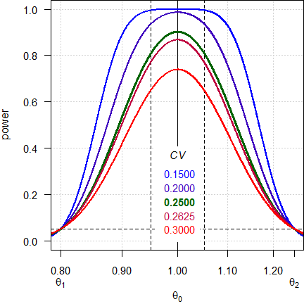
Fig. 1 Power curves for n = 28.
Note the log-scale of the x-axis. It demonstrates that power curves are symmetrical around 1 (\(\small{\log_{e}(1)=0}\), where \(\small{\log_{e}(\theta_2)=\left|\log_{e}(\theta_1)\right|}\)) and we will achieve the same power for \(\small{\theta_0}\) and \(\small{1/\theta_0}\) (e.g., for 0.95 and 1.0526). Furthermore, all curves intersect 0.05 at \(\small{\theta_1}\) and \(\small{\theta_2}\), which means that for a true \(\small{\theta_0}\) at one of the limits the patient’s risk \(\small{\alpha}\) is strictly controlled.
<nitpick>-
A common flaw in protocols is the phrase
»The sample size was calculated [sic] based on a T/R-ratio of 0.95 – 1.05…«
If you assume a deviation of 5% of the test from the reference and are not sure about its direction (lower or higher than 1), always use the lower T/R-ratio. If you would use the upper T/R-ratio, power would be only preserved down to 1/1.05 = 0.9524.
Given, sometimes you will need a higher sample size with the lower T/R-ratio. There’s no free lunch.
CV      <- 0.30
delta   <- 0.05 # direction unknown
theta0s <- c(1 - delta, 1 / (1 + delta),
             1 + delta, 1 / (1 - delta))
n       <- sampleN.TOST(CV = CV, theta0 = 1 - delta,
                        print = FALSE)[["Sample size"]]
comp1   <- data.frame(CV = CV, theta0 = theta0s,
                      base = c(TRUE, rep(FALSE, 3)),
                      n = n, power = NA)
for (i in 1:nrow(comp1)) {
  comp1$power[i] <- power.TOST(CV = CV,
                               theta0 = comp1$theta0[i],
                               n = n)
}
n       <- sampleN.TOST(CV = CV, theta0 = 1 + delta,
                        print = FALSE)[["Sample size"]]
comp2   <- data.frame(CV = CV, theta0 = theta0s,
                      base = c(FALSE, FALSE, TRUE, FALSE),
                      n = n, power = NA)
for (i in 1:nrow(comp2)) {
  comp2$power[i] <- power.TOST(CV = CV,
                               theta0 = comp2$theta0[i],
                               n = n)
}
comp1[, c(2, 5)] <- signif(comp1[, c(2, 5)] , 4)
comp2[, c(2, 5)] <- signif(comp2[, c(2, 5)] , 4)
print(comp1, row.names = FALSE)
print(comp2, row.names = FALSE)
# CV theta0 base n power
# 0.3 0.9500 TRUE 40 0.8158
# 0.3 0.9524 FALSE 40 0.8246
# 0.3 1.0500 FALSE 40 0.8246
# 0.3 1.0530 FALSE 40 0.8158
# CV theta0 base n power
# 0.3 0.9500 FALSE 38 0.7953
# 0.3 0.9524 FALSE 38 0.8043
# 0.3 1.0500 TRUE 38 0.8043
# 0.3 1.0530 FALSE 38 0.7953</nitpick>
Since power is much more sensitive to the T/R-ratio than to the CV, the results obtained with the Bayesian method should be clear now.
Essentially this leads to the murky water of prospective power and sensitivity analyses,
which are covered in other articles.
An appetizer to show the maximum deviations (CV, T/R-ratio and
decreased sample size due to dropouts) which give still a minimum
acceptable power of ≥ 0.70:
CV       <- 0.25
theta0   <- 0.95
target   <- 0.80
minpower <- 0.70
pa       <- pa.ABE(CV = CV, theta0 = theta0,
                   targetpower = target,
                   minpower = minpower)
change.CV     <- 100*(tail(pa$paCV[["CV"]], 1) -
                      pa$plan$CV) / pa$plan$CV
change.theta0 <- 100*(head(pa$paGMR$theta0, 1) -
                      pa$plan$theta0) /
                      pa$plan$theta0
change.n      <- 100*(tail(pa$paN[["N"]], 1) -
                      pa$plan[["Sample size"]]) /
                      pa$plan[["Sample size"]]
comp     <- data.frame(parameter = c("CV", "theta0", "n"),
                       change = c(change.CV,
                                  change.theta0,
                                  change.n))
comp$change <- sprintf("%+.2f%%", comp$change)
names(comp)[2] <- "relative change"
print(pa, plotit = FALSE); print(comp, row.names = FALSE)
# Sample size plan ABE
# Design alpha CV theta0 theta1 theta2 Sample size
# 2x2 0.05 0.25 0.95 0.8 1.25 28
# Achieved power
# 0.8074395
#
# Power analysis
# CV, theta0 and number of subjects leading to min. acceptable power of ~0.7:
# CV= 0.2843, theta0= 0.9268
# n = 23 (power= 0.7173)
#
# parameter relative change
# CV +13.70%
# theta0 -2.44%
# n -17.86%Confirms what we have seen above. Interesting that the sample size is the least sensitive one. Many people overrate the impact of dropouts on power.
If you didn’t stop reading in desperation (understandable), explore both uncertain CV and T/R-ratio:
m      <- 12
CV     <- 0.25
theta0 <- 0.95
expsampleN.TOST(CV = CV, theta0 = theta0,
                targetpower = 0.80,
                design = "2x2",
                prior.parm = list(m = m,
                                  design = "2x2"),
                prior.type = "both", # uncertain CV and T/R-ratio
                details = FALSE)
#
# ++++++++++++ Equivalence test - TOST ++++++++++++
# Sample size est. with uncertain CV and theta0
# -------------------------------------------------
# Study design: 2x2 crossover
# log-transformed data (multiplicative model)
#
# alpha = 0.05, target power = 0.8
# BE margins = 0.8 ... 1.25
# Ratio = 0.95 with 10 df
# CV = 0.25 with 10 df
#
# Sample size (ntotal)
# n exp. power
# 108 0.800126I don’t suggest that you should use it in practice. AFAIK, not even the main author of this function (Benjamin Lang) does. However, it serves educational purposes to show that it is not that easy and why even properly planned studies might fail.
An alternative to assuming a T/R-ratio is based on statistical
assurance.18 This concept uses the distribution of
T/R-ratios and assumes an uncertainty parameter \(\small{\sigma_\textrm{u}}\). A natural
assumption is \(\small{\sigma_\textrm{u}=1-\theta_0}\),
i.e., for the commonly applied T/R-ratio of 0.95 one can use
the argument sem = 0.05 in the function
expsampleN.TOST(), where the argument theta0
has to be fixed at 1.
CV        <- 0.25
theta0    <- 0.95
target    <- 0.80
sigma.u   <- 1 - theta0
comp      <- data.frame(theta0 = theta0,
                        n.1 = NA, power = NA,
                        sigma.u = sigma.u,
                        n.2 = NA, assurance = NA)
comp[2:3] <- sampleN.TOST(CV = CV,
                          targetpower = target,
                          theta0 = theta0,
                          details = FALSE,
                          print = FALSE)[7:8]
comp[5:6] <- expsampleN.TOST(CV = CV,
                             theta0 = 1, # fixed!
                             targetpower = target,
                             design = "2x2",
                             prior.type = "theta0",
                             prior.parm = list(sem = sigma.u),
                             details = FALSE,
                             print = FALSE)[9:10]
names(comp)[c(2, 5)]  <- rep("n", 2)
print(signif(comp, 6), row.names = FALSE)
# theta0 n power sigma.u n assurance
# 0.95 28 0.807439 0.05 28 0.817016Multiple Endpoints
Generally equivalence of more than one endpoint has to be demonstrated. In bioequivalence the PK metrics Cmax and AUC0–t are mandatory (in some jurisdictions like the FDA additionally AUC0–∞).
We don’t have to worry about multiplicity issues (inflated Type I Error) since if all tests must pass at level \(\small{\alpha}\), we are protected by the intersection-union principle.19 20
We design the study always for the worst case combination, i.e., based on the PK metric requiring the largest sample size. In some jurisdictions wider BE limits for Cmax are acceptable. Let’s explore that with different CVs and T/R-ratios.
metrics <- c("Cmax", "AUCt", "AUCinf")
CV      <- c(0.25, 0.19, 0.20)
theta0  <- c(0.95, 1.04, 1.06)
theta1  <- c(0.75, 0.80, 0.80)
theta2  <- 1 / theta1
target  <- 0.80
x       <- data.frame(metric = metrics,
                      theta1 = theta1, theta2 = theta2,
                      CV = CV, theta0 = theta0, n = NA)
for (i in 1:nrow(x)) {
  x$n[i] <- sampleN.TOST(CV = CV[i],
                         theta0 = theta0[i],
                         theta1 = theta1[i],
                         theta2 = theta2[i],
                         targetpower = target,
                         print = FALSE)[["Sample size"]]
}
x$theta1 <- sprintf("%.4f", x$theta1)
x$theta2 <- sprintf("%.4f", x$theta2)
txt       <- paste0("Sample size based on ",
                    x$metric[x$n == max(x$n)], ".\n")
print(x, row.names = FALSE); cat(txt)
# metric theta1 theta2 CV theta0 n
# Cmax 0.7500 1.3333 0.25 0.95 16
# AUCt 0.8000 1.2500 0.19 1.04 16
# AUCinf 0.8000 1.2500 0.20 1.06 20
# Sample size based on AUCinf.Even if we assume the same T/R-ratio for two PK metrics, we will get a wider margin for the one with lower variability.
Let’s continue with the conditions of our previous examples, this time assuming that the CV and T/R-ratio were applicable for Cmax. As common in PK, the CV of AUC is lower, say only 0.20. That means, the study is ‘overpowered’ for the assumed T/R-ratio of AUC.
Which are the extreme T/R-ratios (largest deviations of T from R) giving still the target power?
opt <- function(y) {
  power.TOST(theta0 = y, CV = x$CV[2],
             theta1 = theta1,
             theta2 = theta2,
             n = x$n[1]) - target
}
metrics <- c("Cmax", "AUC")
CV      <- c(0.25, 0.20) # Cmax, AUC
theta0  <- 0.95          # both metrics
theta1  <- 0.80
theta2  <- 1.25
target  <- 0.80
x       <- data.frame(metric = metrics, theta0 = theta0,
                      CV = CV, n = NA, power = NA)
for (i in 1:nrow(x)) {
  x[i, 4:5] <- sampleN.TOST(CV = CV[i],
                            theta0 = theta0,
                            theta1 = theta1,
                            theta2 = theta2,
                            targetpower = target,
                            print = FALSE)[7:8]
}
x$power <- signif(x$power, 6)
if (theta0 < 1) {
  res <- uniroot(opt, tol = 1e-8,
                 interval = c(theta1 + 1e-4, theta0))
} else {
  res <- uniroot(opt, tol = 1e-8,
                 interval = c(theta0, theta2 - 1e-4))
}
res     <- unlist(res)
theta0s <- c(res[["root"]], 1 / res[["root"]])
txt     <- paste0("Target power for ", metrics[2],
                  " and sample size ",
                  x$n[1], "\nachieved for theta0 ",
                  sprintf("%.4f", theta0s[1]), " or ",
                  sprintf("%.4f", theta0s[2]), ".\n")
print(x, row.names = FALSE)
cat(txt)
# metric theta0 CV n power
# Cmax 0.95 0.25 28 0.807439
# AUC 0.95 0.20 20 0.834680
# Target power for AUC and sample size 28
# achieved for theta0 0.9158 or 1.0920.That means, although we assumed for AUC the same T/R-ratio as for Cmax – with the sample size of 28 required for Cmax – for AUC it can be as low as ~0.92 or as high as ~1.09, which is a soothing side-effect.
Furthermore, sometimes we have less data of AUC than of Cmax (samples at the end of the profile missing or unreliable \(\small{\widehat{\lambda}_\textrm{z}}\) in some subjects and therefore, less data of AUC0–∞ than of AUC0–t). Again, it will not hurt because for the originally assumed T/R-ratio we need only 20 subjects.
Since – as a one-point metric – Cmax is
inherently more variable than AUC, Health Canada does not
require assessment of its Confidence Interval. Only the point estimate
has to lie within 80.0 – 125.0%. We can explore that by setting
alpha = 0.5 for it.21
metrics <- c("Cmax", "AUC")
CV      <- c(0.60, 0.20)
theta0  <- 0.95
target  <- 0.80
alpha   <- c(0.50, 0.05)
x       <- data.frame(metric = metrics, CV = CV, theta0 = theta0,
                      alpha = alpha, n = NA_integer_)
for (i in 1:nrow(x)) {
  x$n[i] <- sampleN.TOST(alpha = alpha[i], CV = CV[i],
                         theta0 = theta0, targetpower = target,
                         print = FALSE)[["Sample size"]]
}
txt     <- paste0("Sample size based on ",
                  x$metric[x$n == max(x$n)], ".\n")
print(x, row.names = FALSE)
cat(txt)
# metric CV theta0 alpha n
# Cmax 0.6 0.95 0.50 24
# AUC 0.2 0.95 0.05 20
# Sample size based on Cmax.Only with a relatively high CV (compared to the one of AUC) you may face a situation where you have to base the sample size on Cmax.
NTIDs
So far we employed the common (and hence, default)
BE-limits theta1 = 0.80
and theta2 = 1.25. In some jurisdictions tighter limits of
90.00 – 111.11% have to be used.22
Generally NTIDs show a low within-subject variability (though the between-subject CV can be much higher – these drugs require quite often dose-titration).
You have to provide only the lower
BE-limit theta1 (the
upper one will be automatically calculated as its reciprocal). In the
examples I used a lower CV of 0.125.
#
# +++++++++++ Equivalence test - TOST +++++++++++
#             Sample size estimation
# -----------------------------------------------
# Study design: 2x2 crossover
# log-transformed data (multiplicative model)
#
# alpha = 0.05, target power = 0.8
# BE margins = 0.9 ... 1.111111
# True ratio = 0.95,  CV = 0.125
#
# Sample size (total)
#  n     power
# 68   0.805372
Not so nice. If you would exhaust the capacity of the clinical site, you may consider a replicate design.
Interlude: Health Canada
Health Canada requires for NTIDs (termed by HC ‘critical dose drugs’) that the confidence interval of Cmax lies within 80.0 – 125.0% and the one of AUC within 90.0 – 112.0%.
<nitpick>»These numbers are more easy to remember.«
</nitpick>
Hence, for Health Canada you have to set both limits.
#
# +++++++++++ Equivalence test - TOST +++++++++++
#             Sample size estimation
# -----------------------------------------------
# Study design: 2x2 crossover
# log-transformed data (multiplicative model)
#
# alpha = 0.05, target power = 0.8
# BE margins = 0.9 ... 1.12
# True ratio = 0.95,  CV = 0.125
#
# Sample size (total)
#  n     power
# 68   0.805372
Here we require the same sample size than with the common limits for NTIDs.
If you expect a T/R-ratio closer to 1, possibly you require two subjects less:
target  <- 0.80
theta0  <- 0.975
CV.min  <- 0.075
CV.max  <- 0.20
CV.step <- 1000
CV      <- seq(CV.min, CV.max, length.out = CV.step)
res     <- data.frame(CV = CV, n.EMA = NA_integer_,
                      n.HC = NA_integer_, less = FALSE)
for (i in 1:nrow(res)) {
  res$n.EMA[i] <- sampleN.TOST(CV = CV[i], theta0 = theta0,
                        targetpower = target, design = "2x2",
                        theta1 = 0.90, theta2 = 1/0.90,
                        print = FALSE)[["Sample size"]]
  res$n.HC[i]  <- sampleN.TOST(CV = CV[i], theta0 = theta0,
                        targetpower = target, design = "2x2",
                        theta1 = 0.90, theta2 = 1.12,
                        print = FALSE)[["Sample size"]]
  if (res$n.HC[i] < res$n.EMA[i]) res$less[i] = TRUE
}
cat("target power                :", target,
    "\ntheta0                      :", theta0,
    "\nCV                          :", CV.min, "\u2013", CV.max,
    "\nSample size for HC < common :",
    sprintf("%.2f%% of cases.\n", 100 * sum(res$less) / CV.step))
# target power : 0.8
# theta0 : 0.975
# CV : 0.075 – 0.2
# Sample size for HC < common : 19.40% of cases.The FDA requires for NTIDs tighter batch-release specifications (±5% instead of ±10%). Let’s hope that your product complies and the T/R-ratio will be closer to 1:
#
# +++++++++++ Equivalence test - TOST +++++++++++
#             Sample size estimation
# -----------------------------------------------
# Study design: 2x2 crossover
# log-transformed data (multiplicative model)
#
# alpha = 0.05, target power = 0.8
# BE margins = 0.9 ... 1.111111
# True ratio = 0.975,  CV = 0.125
#
# Sample size (total)
#  n     power
# 32   0.800218
Substantially lower sample size and doable.
Difference of Means
Sometimes we are interested in assessing differences of responses and
not their ratios. In such a case we have to set
logscale = FALSE. The limits theta1 and
theta2 can be expressed in the following ways:
- As a difference of means relative to the same (underlying) reference mean.
- In units of the difference of means.
Note that in the former case the units of CV, and
theta0 need also to be given relative to the reference mean
(specified as ratio).
Let’s estimate the sample size for an equivalence trial of two blood pressure lowering drugs assessing the difference in means of untransformed data (raw, linear scale). In this setup everything has to be given with the same units (i.e., here the assumed difference –5 mm Hg and the lower / upper limits ∓15 mm Hg systolic blood pressure). Furthermore, we assume a CV of 25 mm Hg.
#
# +++++++++++ Equivalence test - TOST +++++++++++
#             Sample size estimation
# -----------------------------------------------
# Study design: 2x2 crossover
# untransformed data (additive model)
#
# alpha = 0.05, target power = 0.8
# BE margins = -15 ... 15
# True diff. = -5,  CV = 25
#
# Sample size (total)
#  n     power
# 80   0.805536
Sometimes in the literature we find not the CV but the standard deviation of the difference \(\small{SD}\). Say, it is given with 35 mm Hg. We have to convert it to a CV. In a 2×2×2 design \(\small{CV=SD/\sqrt{2}}\).
#
# +++++++++++ Equivalence test - TOST +++++++++++
#             Sample size estimation
# -----------------------------------------------
# Study design: 2x2 crossover
# untransformed data (additive model)
#
# alpha = 0.05, target power = 0.8
# BE margins = -15 ... 15
# True diff. = -5,  CV = 24.74874
#
# Sample size (total)
#  n     power
# 78   0.803590
Note that other software packages (e.g., PASS, nQuery, StudySize, …) require the standard deviation of the difference as input.
Ratio of Means
It would be a fundamental flaw if responses are assumed to a follow a normal distribution and not – like above – assess their difference and at the end instead giving an estimate of the difference, calculate the ratio of the test- and reference-means.
In such a case Fieller’s (‘fiducial’) confidence interval23 24 has to
be employed.
Note that alpha = 0.025 is the default in the functions
sampleN.RatioF()and power.RatioF(), since it
is intended for studies with clinical endpoints, where the 95%
confidence interval is usually used for equivalence testing.25 Note
that we need additionally the between-subject CV (in the
example below arbitrarily twice the within-subject CV).
#
# +++++++++++ Equivalence test - TOST +++++++++++
#     based on Fieller's confidence interval
#             Sample size estimation
# -----------------------------------------------
# Study design: 2x2 crossover
# Ratio of means with normality on original scale
# alpha = 0.025, target power = 0.8
# BE margins = 0.8 ... 1.25
# True ratio = 0.95,  CVw = 0.25,  CVb = 0.5
#
# Sample size
#  n     power
# 42 0.802153Methods
“He who seeks for methods without having a definite problem in mind seeks in the most part in vain.
With a few exceptions (i.e., simulation-based methods), in
PowerTOST the default method = "exact"
implements Owen’s Q function26 which is also used in SAS’
Proc Power.
Other implemented methods are "mvt" (based on the
bivariate noncentral t-distribution),
"noncentral" / "nct" (based on the noncentral
t-distribution), and "shifted" /
"central" (based on the shifted central
t-distribution). Although "mvt" is also exact, it
may have a somewhat lower precision compared to Owen’s Q and has a much
longer run-time.
Let’s compare them.
methods <- c("exact", "mvt", "noncentral", "central")
x       <- data.frame(method = methods, power = NA, ms = NA)
for (i in 1:nrow(x)) {
  st <- proc.time()[[3]]
  for (j in 1:1e3L) {# slow it down
    tmp <- power.TOST(CV     = 0.25,
                      n      = 28,
                      method = x$method[i])
    if (j == 1) x$power[i] <- tmp
  }
  x$ms[i] <- sprintf("%.2f", (proc.time()[[3]] - st))
}
print(x, row.names = FALSE)
# method power ms
# exact 0.8074395 0.43
# mvt 0.8074431 94.42
# noncentral 0.8074395 0.29
# central 0.8030251 0.28Power approximated by the shifted central t-distribution is
generally slightly lower compared to the others. Hence, if used in
sample size estimations, occasionally two more subjects are
‘required’ – which is not correct as demonstrated by the exact
method.
Here an example for CV 0.28.
methods <- c("exact", "mvt", "noncentral", "central")
x       <- data.frame(method = methods)
for (i in 1:nrow(x)) {
  tmp               <- sampleN.TOST(CV = 0.28,
                                    theta0 = 0.95,
                                    method = x$method[i],
                                    targetpower = 0.80,
                                    print = FALSE)
  x$n[i]            <- tmp[["Sample size"]]
  x$power.method[i] <- tmp[["Achieved power"]]
  x$power.exact[i]  <- power.TOST(CV = 0.28,
                                   theta0 = 0.95,
                                   n = x$n[i],
                                   method = "exact")
}
print(x, row.names = FALSE)
# method n power.method power.exact
# exact 34 0.8017690 0.8017690
# mvt 34 0.8017720 0.8017690
# noncentral 34 0.8017690 0.8017690
# central 36 0.8210282 0.8242676Particularly for ‘nice’ combinations of the CV and T/R-ratio the relative increase in sample sizes (and hence, study costs) might be relevant.
set.seed(123456)
nsims  <- 1e4
CV     <- signif(runif(nsims, min = 0.13, max = 0.40), 2)
theta0 <- signif(runif(nsims, min = 0.90, max = 0.95), 2)
x      <- data.frame(CV = CV, theta0 = theta0,
                     exact = NA, shifted = NA,
                     diff = NA, delta.n = FALSE)
x      <- unique(x)
for (i in 1:nrow(x)) {
  x$exact[i]   <- sampleN.TOST(CV = x$CV[i],
                               theta0 = x$theta0[i],
                               design = "2x2",
                               method = "exact",
                               print = FALSE)[["Sample size"]]
  x$shifted[i] <- sampleN.TOST(CV = x$CV[i],
                               theta0 = x$theta0[i],
                               design = "2x2",
                               method = "shifted",
                               print = FALSE)[["Sample size"]]
  if (x$shifted[i] != x$exact[i]) x$delta.n[i] <- TRUE
}
x$diff <- 100 * (x$shifted - x$exact) / x$exact
x      <- x[with(x, order(-diff, theta0, CV)), ]
x$diff <- sprintf("%+.3f%%", x$diff)
print(x[which(x$delta.n == TRUE), 1:5], row.names = FALSE)
# CV theta0 exact shifted diff
# 0.14 0.92 14 16 +14.286%
# 0.17 0.95 14 16 +14.286%
# 0.22 0.95 22 24 +9.091%
# 0.19 0.92 24 26 +8.333%
# 0.19 0.91 28 30 +7.143%
# 0.18 0.90 30 32 +6.667%
# 0.28 0.95 34 36 +5.882%
# 0.21 0.90 40 42 +5.000%
# 0.27 0.93 40 42 +5.000%
# 0.27 0.92 46 48 +4.348%
# 0.33 0.95 46 48 +4.348%
# 0.34 0.94 54 56 +3.704%
# 0.36 0.95 54 56 +3.704%
# 0.30 0.92 56 58 +3.571%
# 0.33 0.93 58 60 +3.448%
# 0.36 0.94 60 62 +3.333%
# 0.36 0.93 68 70 +2.941%
# 0.38 0.91 102 104 +1.961%
# 0.36 0.90 110 112 +1.818%
# 0.40 0.91 112 114 +1.786%Therefore, I recommend to use "method = shifted" /
"method = central" only for comparing with old results
(literature, own studies).
Validation
Internal
You can compare the results of sampleN.TOST() to
simulations via the ‘key’ statistics (\(\small{\sigma^2}\) follows a \(\small{\chi^2\textrm{-}}\)distribution with
\(\small{n-2}\) degrees of freedom and
\(\small{\log_{e}(\theta_0)}\) follows
a normal distribution27), which are provided by the function
power.TOST.sim().
In the script 100,000 studies are assessed for BE (where empiric power
is the number of passing studies divided by the number of simulations).
Two sample sizes are tried first: n = 12 and n = 144.
Depending on power, the sample size is increased or decreased until at
least the target power is obtained.
sampleN.key <- function(alpha, CV, theta0, theta1, theta2,
                        targetpower, info = FALSE) {
  # sample size by simulating via the ‘key’ statistics
  opt <- function(x) {
    suppressWarnings(
      suppressMessages(
        power.TOST.sim(alpha = alpha, CV = CV, theta0 = theta0,
                       theta1 = theta1, theta2 = theta2,
                       nsims = nsims, n = x))) - targetpower
  }
  nsims <- 1e5L
  # if you get a substantial difference, increase the number of simulations
  t   <- proc.time()[[3]]
  x   <- uniroot(opt, interval = c(12L, 144L),
                 extendInt = "upX", tol = 0.1)
  if (info) {
    message(signif(proc.time()[[3]] - t, 3), " seconds for ", x$iter,
            " iterations of ", prettyNum(nsims, format = "i", big.mark = ","),
            " simulated  studies.")
  }
  n   <- ceiling(x$root)
  n   <- 2 * (n %/% 2 + as.logical(n %% 2))
  res <- data.frame(alpha = alpha, CV = CV, theta0 = theta0,
                    theta1 = theta1, theta2 = theta2, n = n)
  return(res)
}
internal.validation <- function(alpha, CV, theta0, theta1,
                                theta2, targetpower,
                                info = FALSE) {
  if (missing(alpha)) alpha <- 0.05
  if (missing(CV)) stop("CV must be given!")
  if (missing(theta0)) theta0 <- 0.95
  if (missing(theta1) & missing(theta2)) theta1 <- 0.80
  if (missing(theta1)) theta1 = 1/theta2
  if (missing(theta2)) theta2 = 1/theta1
  if (missing(targetpower)) targetpower <- 0.80
  simulated <- data.frame(Approach = "key",
                          sampleN.key(alpha = alpha, CV = CV, theta0 = theta0,
                                      theta1 = theta1, theta2 = theta2,
                                      targetpower = targetpower,
                                      info = info)[c(2:6)])
  exact     <- data.frame(Approach = "exact",
                          sampleN.TOST(alpha = alpha, CV = CV, theta0 = theta0,
                                       theta1 = theta1, theta2 = theta2,
                                       targetpower = targetpower,
                                       print = FALSE)[c(3:7)])
  names(exact)[6] <- "n"
  comp <- rbind(simulated, exact)
  comp <- cbind(comp, equal = "")
  comp$Approach[1] <- "1: \u2018Key\u2019 statistics"
  comp$Approach[2] <- "2: Exact (Owen\u2019s Q)"
  names(comp)[1]   <- "Sample size estimation"
  if (isTRUE(all.equal(comp$n[2], comp$n[1]))) {
    comp$equal[2]  <- "  yes"
    names(comp)[7] <- "equal?"
  } else {
    comp$equal[2]  <- sprintf("%+3.0f", comp$n[2] - comp$n[1])
    names(comp)[7] <- "diff."
  }
  comp[, 3] <- sprintf("%.4f", comp[, 3])
  comp[, 4] <- sprintf("%.4f", comp[, 4])
  comp[, 5] <- sprintf("%.4f", comp[, 5])
  print(comp, row.names = FALSE, right = FALSE)
}
Example for CV 0.25 (using all defaults).
#  Sample size estimation CV   theta0 theta1 theta2 n  equal?
#  1: ‘Key’ statistics    0.25 0.9500 0.8000 1.2500 28
#  2: Exact (Owen’s Q)    0.25 0.9500 0.8000 1.2500 28   yes
The package contains data frames of sample size tables from the
literature28 29 (show them by typing ct5.1,
ct5.2, ct5.3, and ct5.4.1 in the
R-Console). Execute the script
test_2x2.R in the /tests sub-directory of the
package to reproduce them. If results don’t agree, something went wrong.
Are you still using a version <0.9.3 that is at least thirteen years
old‽ If yes, please update to the current one.
External
You can reproduce the famous ‘Diletti tables’.30 31 Like in
sampleN.TOST() the authors employed Owen’s exact
method26 and eventual odd sample sizes
were rounded up to the next even number. In the papers’ tables such
cases are printed in italics.
Acceptance range 0.8000 – 1.2500:
# Int J Clin Pharmacol Ther Toxicol. 1991; 29(1): 1-8. Table 1
PT0.8 <- Table1a <- data.frame(CV = rep(seq(5, 30, 2.5), 3),
                     Power = rep(c(70, 80, 90), each = 11),
                     TR0.85 = c(10, 16, 28, 42, 60, 80,
                                102, 128, 158, 190, 224,
                                12, 22, 36, 54, 78, 104,
                                134, 168, 206, 248, 292,
                                14, 28, 48, 74, 106, 142,
                                186, 232, 284, 342, 404),
                     TR0.90 = c(6, 6, 10, 14, 18, 22,
                                30, 36, 44, 52, 60,
                                6, 8, 12, 16, 22, 30,
                                38, 46, 56, 68, 80,
                                6, 10, 14, 22, 30, 40,
                                50, 64, 78, 92, 108),
                     TR0.95 = c(4, 6, 6, 8, 10, 12,
                                16, 20, 24, 28, 32,
                                4, 6, 8, 10, 12, 16,
                                20, 24, 28, 34, 40,
                                4, 6, 8, 12, 16, 20,
                                26, 32, 38, 44, 52),
                     TR1.00 = c(4, 4, 6, 8, 10, 12,
                                14, 16, 20, 24, 28,
                                4, 6, 6, 8, 10, 14,
                                16, 20, 24, 28, 32,
                                4, 6, 8, 10, 12, 16,
                                20, 24, 28, 34, 40),
                     TR1.05 = c(4, 6, 6, 8, 10, 12,
                                16, 20, 22, 26, 32,
                                4, 6, 8, 10, 12, 16,
                                18, 24, 28, 34, 38,
                                4, 6, 8, 12, 16, 20,
                                24, 30, 36, 44, 52),
                     TR1.10 = c(4, 6, 8, 12, 16, 20,
                                26, 30, 38, 44, 52,
                                6, 8, 10, 14, 20, 26,
                                32, 40, 48, 58, 68,
                                6, 8, 14, 18, 26, 34,
                                44, 54, 66, 78, 92),
                     TR1.15 = c(6, 10, 16, 24, 32, 44,
                                56, 70, 84, 102, 120,
                                8, 12, 20, 30, 42, 56,
                                72, 90, 110, 132, 156,
                                8, 16, 26, 40, 58, 76,
                                100, 124, 152, 182, 214),
                     TR1.20 = c(16, 34, 58, 90, 128, 172,
                                224, 282, 344, 414, 490,
                                22, 44, 76, 118, 168, 226,
                                294, 368, 452, 544, 642,
                                28, 60, 104, 162, 232, 312,
                                406, 510, 626, 752, 888))
PT0.8[, 3:ncol(PT0.8)] <- NA_integer_
for (i in 1:nrow(PT0.8)) {
  PT0.8$TR0.85[i] <- sampleN.TOST(CV = PT0.8$CV[i] / 100,
                                   theta0 = 0.85,
                                   targetpower = PT0.8$Power[i] / 100,
                                   print = FALSE)[["Sample size"]]
  PT0.8$TR0.90[i] <- sampleN.TOST(CV = PT0.8$CV[i] / 100,
                                   theta0 = 0.9,
                                   targetpower = PT0.8$Power[i] / 100,
                                   print = FALSE)[["Sample size"]]
  PT0.8$TR0.95[i] <- sampleN.TOST(CV = PT0.8$CV[i] / 100,
                                   theta0 = 0.95,
                                   targetpower = PT0.8$Power[i] / 100,
                                   print = FALSE)[["Sample size"]]
  PT0.8$TR1.00[i] <- sampleN.TOST(CV = PT0.8$CV[i] / 100,
                                   theta0 = 1,
                                   targetpower = PT0.8$Power[i] / 100,
                                   print = FALSE)[["Sample size"]]
  PT0.8$TR1.05[i] <- sampleN.TOST(CV = PT0.8$CV[i] / 100,
                                   theta0 = 1.05,
                                   targetpower = PT0.8$Power[i] / 100,
                                   print = FALSE)[["Sample size"]]
  PT0.8$TR1.10[i] <- sampleN.TOST(CV = PT0.8$CV[i] / 100,
                                   theta0 = 1.1,
                                   targetpower = PT0.8$Power[i] / 100,
                                   print = FALSE)[["Sample size"]]
  PT0.8$TR1.15[i] <- sampleN.TOST(CV = PT0.8$CV[i] / 100,
                                   theta0 = 1.15,
                                   targetpower = PT0.8$Power[i] / 100,
                                   print = FALSE)[["Sample size"]]
  PT0.8$TR1.20[i] <- sampleN.TOST(CV = PT0.8$CV[i] / 100,
                                   theta0 = 1.20,
                                   targetpower = PT0.8$Power[i] / 100,
                                   print = FALSE)[["Sample size"]]
}

if (!sum(PT0.8 - Table1a) == 0) {
  cat("Failed checking Table 1: 0.8000 \u2013 1.2500, powers 70, 80, and 90%. Discrepancies:\n")
  comp <- comparedf(PT0.8, Table1a)
  cols <- diffs(comp)[[1]]
  d    <- data.frame(
            type.convert(
              comp$vars.summary$values[[3]][-c(4:5)], as.is = FALSE))
  names(d) <- c("CV", "estimated", "reported")
  for (i in 1:nrow(d)) {
    d$CV    <- Table1a$CV[d$CV[i]]
    d[i, 2] <- paste(cols, "=", d[i, 2])
    d[i, 3] <- paste(cols, "=", d[i, 3])
  }
  names(d)[1] <- "CV (%)"
  print(d, row.names = FALSE)
} else {
  cat("Passed checking Table 1: 0.8000 \u2013 1.2500, powers 70, 80, and 90%.\n")
}
names(PT0.8)[1:2] <- c("CV (%)", "Power (%)")
print(PT0.8[, 1:6], row.names = FALSE)
print(PT0.8[, c(1:2, 7:10)], row.names = FALSE)
# Passed checking Table 1: 0.8000 – 1.2500, powers 70, 80, and 90%.
# CV (%) Power (%) TR0.85 TR0.90 TR0.95 TR1.00
# 5.0 70 10 6 4 4
# 7.5 70 16 6 6 4
# 10.0 70 28 10 6 6
# 12.5 70 42 14 8 8
# 15.0 70 60 18 10 10
# 17.5 70 80 22 12 12
# 20.0 70 102 30 16 14
# 22.5 70 128 36 20 16
# 25.0 70 158 44 24 20
# 27.5 70 190 52 28 24
# 30.0 70 224 60 32 28
# 5.0 80 12 6 4 4
# 7.5 80 22 8 6 6
# 10.0 80 36 12 8 6
# 12.5 80 54 16 10 8
# 15.0 80 78 22 12 10
# 17.5 80 104 30 16 14
# 20.0 80 134 38 20 16
# 22.5 80 168 46 24 20
# 25.0 80 206 56 28 24
# 27.5 80 248 68 34 28
# 30.0 80 292 80 40 32
# 5.0 90 14 6 4 4
# 7.5 90 28 10 6 6
# 10.0 90 48 14 8 8
# 12.5 90 74 22 12 10
# 15.0 90 106 30 16 12
# 17.5 90 142 40 20 16
# 20.0 90 186 50 26 20
# 22.5 90 232 64 32 24
# 25.0 90 284 78 38 28
# 27.5 90 342 92 44 34
# 30.0 90 404 108 52 40
# CV (%) Power (%) TR1.05 TR1.10 TR1.15 TR1.20
# 5.0 70 4 4 6 16
# 7.5 70 6 6 10 34
# 10.0 70 6 8 16 58
# 12.5 70 8 12 24 90
# 15.0 70 10 16 32 128
# 17.5 70 12 20 44 172
# 20.0 70 16 26 56 224
# 22.5 70 20 30 70 282
# 25.0 70 22 38 84 344
# 27.5 70 26 44 102 414
# 30.0 70 32 52 120 490
# 5.0 80 4 6 8 22
# 7.5 80 6 8 12 44
# 10.0 80 8 10 20 76
# 12.5 80 10 14 30 118
# 15.0 80 12 20 42 168
# 17.5 80 16 26 56 226
# 20.0 80 18 32 72 294
# 22.5 80 24 40 90 368
# 25.0 80 28 48 110 452
# 27.5 80 34 58 132 544
# 30.0 80 38 68 156 642
# 5.0 90 4 6 8 28
# 7.5 90 6 8 16 60
# 10.0 90 8 14 26 104
# 12.5 90 12 18 40 162
# 15.0 90 16 26 58 232
# 17.5 90 20 34 76 312
# 20.0 90 24 44 100 406
# 22.5 90 30 54 124 510
# 25.0 90 36 66 152 626
# 27.5 90 44 78 182 752
# 30.0 90 52 92 214 888Acceptance range 0.9000 – 1.1111:
# Int J Clin Pharmacol Ther Toxicol. 1992; 30(Suppl1): S59-62. Table 1
PT0.9 <- Table1b <- data.frame(CV = rep(seq(5, 20, 2.5), 3),
                     Power = rep(c(70, 80, 90), each = 7),
                     TR0.925 = c(34, 72, 128, 196, 282,380, 494,
                                 44, 94, 166, 258, 368, 500, 648,
                                 60, 130, 230, 356, 510, 690, 898),
                     TR0.950 = c(10, 20, 34, 52, 74, 100, 128,
                                 14, 26, 44, 68, 96, 130, 168,
                                 18, 36, 60, 94, 132, 180, 232),
                     TR0.975 = c(6, 12, 18, 26, 38, 50, 64,
                                 8, 14, 22, 32, 46, 62, 80,
                                 10, 18, 30, 44, 62, 84, 108),
                     TR1.000 = c(6, 10, 16, 22, 32, 42, 54,
                                 6, 12, 18, 26, 36, 48, 62,
                                 8, 14, 22, 32, 46, 62, 78),
                     TR1.025 = c(6, 12, 18, 26, 36, 48, 62,
                                 8, 14, 22, 32, 46, 62, 78,
                                 10, 18, 28, 44, 62, 82, 106),
                     TR1.050 = c(10, 20, 32, 48, 68, 92, 118,
                                 12, 24, 40, 62, 88, 118, 154,
                                 16, 32, 56, 86, 122, 164, 212),
                     TR1.075 = c(24, 50, 88, 136, 194, 262, 340,
                                 30, 66, 116, 178, 254, 344, 446,
                                 42, 90, 158, 246, 352, 476, 618))
PT0.9[, 3:ncol(PT0.9)] <- NA_integer_
for (i in 1:nrow(PT0.9)) {
  PT0.9$TR0.925[i] <- sampleN.TOST(CV = PT0.9$CV[i] / 100,
                                   theta0 = 0.925,
                                   theta1 = 0.9, theta2 = 1.1111,
                                   targetpower = PT0.9$Power[i] / 100,
                                   print = FALSE)[["Sample size"]]
  PT0.9$TR0.950[i] <- sampleN.TOST(CV = PT0.9$CV[i] / 100,
                                   theta0 = 0.950,
                                   theta1 = 0.9, theta2 = 1.1111,
                                   targetpower = PT0.9$Power[i] / 100,
                                   print = FALSE)[["Sample size"]]
  PT0.9$TR0.975[i] <- sampleN.TOST(CV = PT0.9$CV[i] / 100,
                                   theta0 = 0.975,
                                   theta1 = 0.9, theta2 = 1.1111,
                                   targetpower = PT0.9$Power[i] / 100,
                                   print = FALSE)[["Sample size"]]
  PT0.9$TR1.000[i] <- sampleN.TOST(CV = PT0.9$CV[i] / 100,
                                   theta0 = 1,
                                   theta1 = 0.9, theta2 = 1.1111,
                                   targetpower = PT0.9$Power[i] / 100,
                                   print = FALSE)[["Sample size"]]
  PT0.9$TR1.025[i] <- sampleN.TOST(CV = PT0.9$CV[i] / 100,
                                   theta0 = 1.025,
                                   theta1 = 0.9, theta2 = 1.1111,
                                   targetpower = PT0.9$Power[i] / 100,
                                   print = FALSE)[["Sample size"]]
  PT0.9$TR1.050[i] <- sampleN.TOST(CV = PT0.9$CV[i] / 100,
                                   theta0 = 1.05,
                                   theta1 = 0.9, theta2 = 1.1111,
                                   targetpower = PT0.9$Power[i] / 100,
                                   print = FALSE)[["Sample size"]]
  PT0.9$TR1.075[i] <- sampleN.TOST(CV = PT0.9$CV[i] / 100,
                                   theta0 = 1.075,
                                   theta1 = 0.9, theta2 = 1.1111,
                                   targetpower = PT0.9$Power[i] / 100,
                                   print = FALSE)[["Sample size"]]
}
if (!sum(PT0.9 - Table1b) == 0) {
  cat("Failed checking Table 1: 0.9000 \u2013 1.1111, powers 70, 80, and 90%. Discrepancies:\n")
  comp <- comparedf(PT0.9, Table1b)
  cols <- diffs(comp)[[1]]
  d    <- data.frame(
            type.convert(
              comp$vars.summary$values[[3]][-c(4:5)], as.is = FALSE))
  names(d) <- c("CV", "estimated", "reported")
  for (i in 1:nrow(d)) {
    d$CV    <- Table1b$CV[d$CV[i]]
    d[i, 2] <- paste(cols, "=", d[i, 2])
    d[i, 3] <- paste(cols, "=", d[i, 3])
  }
  names(d)[1] <- "CV (%)"
  print(d, row.names = FALSE)
} else {
  cat("Passed checking Table 1: 0.9000 \u2013 1.1111, powers 70, 80, and 90%.\n")
}
names(PT0.9)[1:2] <- c("CV (%)", "Power (%)")
print(PT0.9[, 1:6], row.names = FALSE)
print(PT0.9[, c(1:2, 7:8)], row.names = FALSE)
# Passed checking Table 1: 0.9000 – 1.1111, powers 70, 80, and 90%.
# CV (%) Power (%) TR0.925 TR0.950 TR0.975 TR1.000
# 5.0 70 34 10 6 6
# 7.5 70 72 20 12 10
# 10.0 70 128 34 18 16
# 12.5 70 196 52 26 22
# 15.0 70 282 74 38 32
# 17.5 70 380 100 50 42
# 20.0 70 494 128 64 54
# 5.0 80 44 14 8 6
# 7.5 80 94 26 14 12
# 10.0 80 166 44 22 18
# 12.5 80 258 68 32 26
# 15.0 80 368 96 46 36
# 17.5 80 500 130 62 48
# 20.0 80 648 168 80 62
# 5.0 90 60 18 10 8
# 7.5 90 130 36 18 14
# 10.0 90 230 60 30 22
# 12.5 90 356 94 44 32
# 15.0 90 510 132 62 46
# 17.5 90 690 180 84 62
# 20.0 90 898 232 108 78
# CV (%) Power (%) TR1.025 TR1.050
# 5.0 70 6 10
# 7.5 70 12 20
# 10.0 70 18 32
# 12.5 70 26 48
# 15.0 70 36 68
# 17.5 70 48 92
# 20.0 70 62 118
# 5.0 80 8 12
# 7.5 80 14 24
# 10.0 80 22 40
# 12.5 80 32 62
# 15.0 80 46 88
# 17.5 80 62 118
# 20.0 80 78 154
# 5.0 90 10 16
# 7.5 90 18 32
# 10.0 90 28 56
# 12.5 90 44 86
# 15.0 90 62 122
# 17.5 90 82 164
# 20.0 90 106 212Acceptance range 0.7000 – 1.4286 (of historical interest, included for completeness only):
# Int J Clin Pharmacol Ther Toxicol. 1992; 30(Suppl1): S59-62. Table 2
PT0.7 <- Table2 <- data.frame(CV = rep(seq(15, 60, 5), 3),
                     Power = rep(c(70, 80, 90), each = 10),
                     TR0.75 = c(46, 80, 122, 172, 230,
                                296, 366, 444, 524, 610,
                                60, 104, 160, 226, 302,
                                388, 482, 582, 688, 802,
                                82, 144, 220, 312, 418,
                                536, 666, 806, 954, 1108),
                     TR0.80 = c(14, 24, 34, 48, 64,
                                80, 100, 120, 142, 164,
                                18, 30, 44, 62, 82, 106,
                                130, 158, 186, 216,
                                24, 40, 60, 86, 114,
                                144, 180, 216, 256, 298),
                     TR0.85 = c(8, 12, 18, 24, 32,
                                40, 48, 58, 68, 80,
                                10, 16, 22, 30, 40,
                                52, 62, 76, 90, 104,
                                12, 20, 30, 42, 54,
                                70, 86, 104, 122, 142),
                     TR0.90 = c(6, 8, 12, 16, 20,
                                26, 30, 36, 42, 50,
                                8, 10, 14, 20, 26,
                                32, 38, 46, 54, 62,
                                8, 14, 18, 26, 34,
                                42, 52, 62, 74, 86),
                     TR0.95 = c(6, 8, 10, 12, 16,
                                20, 24, 30, 34, 40,
                                6, 8, 12, 16, 20,
                                24, 30, 36, 42, 48,
                                8, 10, 14, 18, 24,
                                30, 38, 46, 52, 62),
                     TR1.00 = c(6, 8, 10, 12, 16,
                                20, 24, 28, 32, 38,
                                6, 8, 10, 14, 18,
                                22, 28, 32, 38, 44,
                                6, 10, 12, 18, 22,
                                28, 34, 40, 48, 54),
                     TR1.05 = c(6, 8, 10, 12, 16,
                                20, 24, 30, 34, 40,
                                6, 8, 12, 16, 20,
                                24, 30, 34, 40, 46,
                                8, 10, 14, 18, 24,
                                30, 38, 44, 52, 60),
                     TR1.10 = c(6, 8, 12, 14, 20,
                                24, 28, 34, 40, 46,
                                8, 10, 14, 18, 24,
                                30, 36, 44, 50, 58,
                                8, 12, 18, 24, 32,
                                40, 48, 58, 68, 80),
                     TR1.15 = c(8, 10, 14, 20, 26,
                                32, 40, 48, 56, 64,
                                8, 12, 18, 26, 32,
                                42, 50, 62, 72, 84,
                                10, 16, 24, 34, 44,
                                56, 70, 84, 98, 114),
                     TR1.20 = c(10, 14, 22, 30, 38,
                                48, 60, 72, 84, 98,
                                12, 18, 28, 38, 50,
                                62, 78, 94, 110, 128,
                                16, 24, 36, 50, 68,
                                86, 106, 128, 152, 176),
                     TR1.25 = c(14, 24, 34, 48, 64,
                                80, 100, 120, 142, 164,
                                18, 30, 44, 62, 82,
                                106, 130, 158, 186, 216,
                                24, 40, 60, 86, 114,
                                144, 180, 216, 256, 298),
                     TR1.30 = c(26, 44, 66, 94, 124,
                                160, 198, 238, 282, 328,
                                34, 56, 86, 122, 162,
                                208, 258, 312, 370, 430,
                                46, 78, 120, 168, 224,
                                288, 358, 432, 512, 594),
                     TR1.35 = c(68, 118, 180, 256, 342,
                                438, 544, 658, 780, 906,
                                88, 154, 236, 336, 448,
                                576, 714, 864, 1022, 1190,
                                122, 212, 326, 464, 620,
                                796, 988, 1196, 1416, 1646))
PT0.7[, 3:ncol(PT0.7)] <- NA_integer_
for (i in 1:nrow(PT0.7)) {
  PT0.7$TR0.75[i] <- sampleN.TOST(CV = PT0.7$CV[i] / 100,
                                  theta0 = 0.75,
                                  theta1 = 0.7, theta2 = 1.4286,
                                  targetpower = PT0.7$Power[i] / 100,
                                  print = FALSE)[["Sample size"]]
  PT0.7$TR0.80[i] <- sampleN.TOST(CV = PT0.7$CV[i] / 100,
                                  theta0 = 0.80,
                                  theta1 = 0.7, theta2 = 1.4286,
                                  targetpower = PT0.7$Power[i] / 100,
                                  print = FALSE)[["Sample size"]]
  PT0.7$TR0.85[i] <- sampleN.TOST(CV = PT0.7$CV[i] / 100,
                                  theta0 = 0.85,
                                  theta1 = 0.7, theta2 = 1.4286,
                                 targetpower = PT0.7$Power[i] / 100,
                                  print = FALSE)[["Sample size"]]
  PT0.7$TR0.90[i] <- sampleN.TOST(CV = PT0.7$CV[i] / 100,
                                  theta0 = 0.9,
                                  theta1 = 0.7, theta2 = 1.4286,
                                  targetpower = PT0.7$Power[i] / 100,
                                  print = FALSE)[["Sample size"]]
  PT0.7$TR0.95[i] <- sampleN.TOST(CV = PT0.7$CV[i] / 100,
                                  theta0 = 0.95,
                                  theta1 = 0.7, theta2 = 1.4286,
                                  targetpower = PT0.7$Power[i] / 100,
                                  print = FALSE)[["Sample size"]]
  PT0.7$TR1.00[i] <- sampleN.TOST(CV = PT0.7$CV[i] / 100,
                                  theta0 = 1,
                                  theta1 = 0.7, theta2 = 1.4286,
                                  targetpower = PT0.7$Power[i] / 100,
                                  print = FALSE)[["Sample size"]]
  PT0.7$TR1.05[i] <- sampleN.TOST(CV = PT0.7$CV[i] / 100,
                                  theta0 = 1.05,
                                  theta1 = 0.7, theta2 = 1.4286,
                                  targetpower = PT0.7$Power[i] / 100,
                                  method = "nct",
                                  print = FALSE)[["Sample size"]]
  PT0.7$TR1.10[i] <- sampleN.TOST(CV = PT0.7$CV[i] / 100,
                                  theta0 = 1.1,
                                  theta1 = 0.7, theta2 = 1.4286,
                                  targetpower = PT0.7$Power[i] / 100,
                                  print = FALSE)[["Sample size"]]
  PT0.7$TR1.15[i] <- sampleN.TOST(CV = PT0.7$CV[i] / 100,
                                  theta0 = 1.15,
                                  theta1 = 0.7, theta2 = 1.4286,
                                  targetpower = PT0.7$Power[i] / 100,
                                  print = FALSE)[["Sample size"]]
  PT0.7$TR1.20[i] <- sampleN.TOST(CV = PT0.7$CV[i] / 100,
                                  theta0 = 1.2,
                                  theta1 = 0.7, theta2 = 1.4286,
                                  targetpower = PT0.7$Power[i] / 100,
                                  print = FALSE)[["Sample size"]]
  PT0.7$TR1.25[i] <- sampleN.TOST(CV = PT0.7$CV[i] / 100,
                                  theta0 = 1.25,
                                  theta1 = 0.7, theta2 = 1.4286,
                                  targetpower = PT0.7$Power[i] / 100,
                                  print = FALSE)[["Sample size"]]
  PT0.7$TR1.30[i] <- sampleN.TOST(CV = PT0.7$CV[i] / 100,
                                  theta0 = 1.3,
                                  theta1 = 0.7, theta2 = 1.4286,
                                  targetpower = PT0.7$Power[i] / 100,
                                  print = FALSE)[["Sample size"]]
  PT0.7$TR1.35[i] <- sampleN.TOST(CV = PT0.7$CV[i] / 100,
                                  theta0 = 1.35,
                                  theta1 = 0.7, theta2 = 1.4286,
                                  targetpower = PT0.7$Power[i] / 100,
                                  print = FALSE)[["Sample size"]]
}
if (!sum(PT0.7 - Table2) == 0) {
  cat("Failed checking Table 2: 0.7000 \u2013 1.4286, powers 70, 80, and 90%. Discrepancies:\n")
  comp <- comparedf(PT0.7, Table2)
  cols <- diffs(comp)[[1]]
  d    <- data.frame(
            type.convert(
              comp$vars.summary$values[[3]][-c(4:5)], as.is = FALSE))
  names(d) <- c("CV", "estimated", "reported")
  for (i in 1:nrow(d)) {
    d$CV    <- Table2$CV[d$CV[i]]
    d[i, 2] <- paste(cols, "=", d[i, 2])
    d[i, 3] <- paste(cols, "=", d[i, 3])
  }
  names(d)[1] <- "CV (%)"
  print(d, row.names = FALSE)
} else {
  cat("Passed checking Table 2: 0.7000 \u2013 1.4286, powers 70, 80, and 90%.\n")
}
names(PT0.7)[1:2] <- c("CV (%)", "Power (%)")
print(PT0.7[, 1:8], row.names = FALSE)
print(PT0.7[, c(1:2, 9:15)], row.names = FALSE)
# Passed checking Table 2: 0.7000 – 1.4286, powers 70, 80, and 90%.
# CV (%) Power (%) TR0.75 TR0.80 TR0.85 TR0.90 TR0.95 TR1.00
# 15 70 46 14 8 6 6 6
# 20 70 80 24 12 8 8 8
# 25 70 122 34 18 12 10 10
# 30 70 172 48 24 16 12 12
# 35 70 230 64 32 20 16 16
# 40 70 296 80 40 26 20 20
# 45 70 366 100 48 30 24 24
# 50 70 444 120 58 36 30 28
# 55 70 524 142 68 42 34 32
# 60 70 610 164 80 50 40 38
# 15 80 60 18 10 8 6 6
# 20 80 104 30 16 10 8 8
# 25 80 160 44 22 14 12 10
# 30 80 226 62 30 20 16 14
# 35 80 302 82 40 26 20 18
# 40 80 388 106 52 32 24 22
# 45 80 482 130 62 38 30 28
# 50 80 582 158 76 46 36 32
# 55 80 688 186 90 54 42 38
# 60 80 802 216 104 62 48 44
# 15 90 82 24 12 8 8 6
# 20 90 144 40 20 14 10 10
# 25 90 220 60 30 18 14 12
# 30 90 312 86 42 26 18 18
# 35 90 418 114 54 34 24 22
# 40 90 536 144 70 42 30 28
# 45 90 666 180 86 52 38 34
# 50 90 806 216 104 62 46 40
# 55 90 954 256 122 74 52 48
# 60 90 1108 298 142 86 62 54
# CV (%) Power (%) TR1.05 TR1.10 TR1.15 TR1.20 TR1.25 TR1.30 TR1.35
# 15 70 6 6 8 10 14 26 68
# 20 70 8 8 10 14 24 44 118
# 25 70 10 12 14 22 34 66 180
# 30 70 12 14 20 30 48 94 256
# 35 70 16 20 26 38 64 124 342
# 40 70 20 24 32 48 80 160 438
# 45 70 24 28 40 60 100 198 544
# 50 70 30 34 48 72 120 238 658
# 55 70 34 40 56 84 142 282 780
# 60 70 40 46 64 98 164 328 906
# 15 80 6 8 8 12 18 34 88
# 20 80 8 10 12 18 30 56 154
# 25 80 12 14 18 28 44 86 236
# 30 80 16 18 26 38 62 122 336
# 35 80 20 24 32 50 82 162 448
# 40 80 24 30 42 62 106 208 576
# 45 80 30 36 50 78 130 258 714
# 50 80 34 44 62 94 158 312 864
# 55 80 40 50 72 110 186 370 1022
# 60 80 46 58 84 128 216 430 1190
# 15 90 8 8 10 16 24 46 122
# 20 90 10 12 16 24 40 78 212
# 25 90 14 18 24 36 60 120 326
# 30 90 18 24 34 50 86 168 464
# 35 90 24 32 44 68 114 224 620
# 40 90 30 40 56 86 144 288 796
# 45 90 38 48 70 106 180 358 988
# 50 90 44 58 84 128 216 432 1196
# 55 90 52 68 98 152 256 512 1416
# 60 90 60 80 114 176 298 594 1646Sample sizes are also given by Jackson.32 The tables were provided by Volker Steinijans and Edgar Diletti employing Owen’s exact method.26
# Table 1-4: 90 to 111%, powers 0.8 and 0.9
PT0.9 <- Table1.4 <- data.frame(CV = rep(seq(10, 40, 5), 2),
                                Power = rep(c(0.8, 0.9), each = 7),
                                TR0.92 = c(258, 572, 1006, 1554, 2208, 2960, 3802,
                                           356, 792, 1392, 2152, 3058, 4100, 5264),
                                TR0.94 = c(68, 148, 258, 398, 566, 758, 972,
                                           92, 204, 358, 552, 782, 1050, 1346),
                                TR0.96 = c(32, 68, 118, 182, 258, 346, 444,
                                           44, 94, 164, 252, 356, 478, 612),
                                TR0.98 = c(20, 42, 72, 112, 156, 210, 268,
                                           26, 56, 96, 148, 208, 280, 358),
                                TR1.00 = c(18, 36, 62, 96, 136, 180, 232,
                                           22, 46, 78, 120, 170, 228, 292))
PT0.9[, 3:ncol(PT0.9)] <- NA_integer_
for (i in 1:nrow(PT0.9)) {
  PT0.9$TR0.92[i] <- sampleN.TOST(CV = PT0.9$CV[i] / 100, theta0 = 0.92,
                                  theta1 = 0.9, targetpower = PT0.9$Power[i],
                                  print = FALSE)[["Sample size"]]
  PT0.9$TR0.94[i] <- sampleN.TOST(CV = PT0.9$CV[i] / 100, theta0 = 0.94,
                                  theta1 = 0.9, targetpower = PT0.9$Power[i],
                                  print = FALSE)[["Sample size"]]
  PT0.9$TR0.96[i] <- sampleN.TOST(CV = PT0.9$CV[i] / 100, theta0 = 0.96,
                                  theta1 = 0.9, targetpower = PT0.9$Power[i],
                                  print = FALSE)[["Sample size"]]
  PT0.9$TR0.98[i] <- sampleN.TOST(CV = PT0.9$CV[i] / 100, theta0 = 0.98,
                                  theta1 = 0.9, targetpower = PT0.9$Power[i],
                                  print = FALSE)[["Sample size"]]
  PT0.9$TR1.00[i] <- sampleN.TOST(CV = PT0.9$CV[i] / 100, theta0 = 1,
                                  theta1 = 0.9, targetpower = PT0.9$Power[i],
                                  print = FALSE)[["Sample size"]]
}
if (!sum(PT0.9 - Table1.4) == 0) {
  cat("Failed checking Table 1-4: 90 to 111%, powers 0.8 and 0.9. Discrepancies:\n")
  comp <- comparedf(PT0.8, Table1.5)
  cols <- diffs(comp)[[1]]
  d    <- data.frame(
            type.convert(
              comp$vars.summary$values[[3]][-c(4:5)], as.is = FALSE))
  names(d) <- c("CV", "estimated", "reported")
  for (i in 1:nrow(d)) {
    d$CV    <- Table1.4$CV[d$CV[i]]
    d[i, 2] <- paste(cols, "=", d[i, 2])
    d[i, 3] <- paste(cols, "=", d[i, 3])
  }
  names(d)[1] <- "CV (%)"
  print(d, row.names = FALSE)
} else {
  cat("Passed checking Table 1-4: 90 to 111%, powers 0.8 and 0.9.\n")
}
names(PT0.9)[1:2] <- c("CV (%)", "Power (%)")
print(PT0.9, row.names = FALSE)
# Passed checking Table 1-4: 90 to 111%, powers 0.8 and 0.9.
# CV (%) Power (%) TR0.92 TR0.94 TR0.96 TR0.98 TR1.00
# 10 0.8 258 68 32 20 18
# 15 0.8 572 148 68 42 36
# 20 0.8 1006 258 118 72 62
# 25 0.8 1554 398 182 112 96
# 30 0.8 2208 566 258 156 136
# 35 0.8 2960 758 346 210 180
# 40 0.8 3802 972 444 268 232
# 10 0.9 356 92 44 26 22
# 15 0.9 792 204 94 56 46
# 20 0.9 1392 358 164 96 78
# 25 0.9 2152 552 252 148 120
# 30 0.9 3058 782 356 208 170
# 35 0.9 4100 1050 478 280 228
# 40 0.9 5264 1346 612 358 292# Table 1-5: 80 to 125%, powers 0.8 and 0.9
PT0.8 <- Table1.5 <- data.frame(CV = rep(seq(10, 40, 5), 2),
Power = rep(c(0.8, 0.9), each = 7),
TR0.85 = c(36, 78, 134, 206, 292, 392, 502,
48, 106, 186, 284, 404, 540, 694),
TR0.90 = c(12, 22, 38, 56, 80, 106, 134,
14, 30, 50, 78, 108, 146, 186),
TR0.95 = c(8, 12, 26, 28, 40, 52, 66,
8, 16, 20, 38, 52, 70, 88),
TR1.00 = c(6, 10, 16, 24, 32, 42, 54,
8, 12, 20, 28, 40, 52, 66))
PT0.8[, 3:ncol(PT0.8)] <- NA_integer_
for (i in 1:nrow(PT0.8)) {
PT0.8$TR0.85[i] <- sampleN.TOST(CV = PT0.8$CV[i] / 100, theta0 = 0.85,
targetpower = PT0.8$Power[i],
print = FALSE)[["Sample size"]]
PT0.8$TR0.90[i] <- sampleN.TOST(CV = PT0.8$CV[i] / 100, theta0 = 0.9,
targetpower = PT0.8$Power[i],
print = FALSE)[["Sample size"]]
PT0.8$TR0.95[i] <- sampleN.TOST(CV = PT0.8$CV[i] / 100, theta0 = 0.95,
targetpower = PT0.8$Power[i],
print = FALSE)[["Sample size"]]
PT0.8$TR1.00[i] <- sampleN.TOST(CV = PT0.8$CV[i] / 100, theta0 = 1,
targetpower = PT0.8$Power[i],
print = FALSE)[["Sample size"]]
}
if (!sum(PT0.8 - Table1.5) == 0) {
cat("Failed checking Table 1-5: 80 to 125%, powers 0.8 and 0.9. Discrepancies:\n")
comp <- comparedf(PT0.8, Table1.5)
cols <- diffs(comp)[[1]]
d <- data.frame(
type.convert(
comp$vars.summary$values[[3]][-c(4:5)], as.is = FALSE))
names(d) <- c("CV", "estimated", "reported")
for (i in 1:nrow(d)) {
d$CV <- Table1.5$CV[d$CV[i]]
d[i, 2] <- paste(cols, "=", d[i, 2])
d[i, 3] <- paste(cols, "=", d[i, 3])
}
names(d)[1] <- "CV (%)"
print(d, row.names = FALSE)
} else {
cat("Passed checking Table 1-5: 80 to 125%, powers 0.8 and 0.9.\n")
}
names(PT0.8)[1] <- "CV (%)"
print(PT0.8, row.names = FALSE)# Passed checking Table 1-5: 80 to 125%, powers 0.8 and 0.9.
# CV (%) Power TR0.85 TR0.90 TR0.95 TR1.00
# 10 0.8 36 12 8 6
# 15 0.8 78 22 12 10
# 20 0.8 134 38 20 16
# 25 0.8 206 56 28 24
# 30 0.8 292 80 40 32
# 35 0.8 392 106 52 42
# 40 0.8 502 134 66 54
# 10 0.9 48 14 8 8
# 15 0.9 106 30 16 12
# 20 0.9 186 50 26 20
# 25 0.9 284 78 38 28
# 30 0.9 404 108 52 40
# 35 0.9 540 146 70 52
# 40 0.9 694 186 88 66# Table 1-6: 70 to 143%, powers 0.8 and 0.9
PT0.7 <- Table1.6 <- data.frame(CV = rep(seq(10, 40, 5), 2),
Power = rep(c(0.8, 0.9), each = 7),
TR0.75 = c(28, 60, 204, 160, 226, 302, 388,
38, 82, 144, 220, 312, 418, 536),
TR0.80 = c(10, 18, 30, 44, 62, 82, 106,
12, 24, 40, 60, 86, 114, 144),
TR0.85 = c(6, 10, 16, 22, 30, 40, 52,
8, 12, 20, 30, 42, 54, 70),
TR0.90 = c(6, 8, 10, 14, 20, 26, 32,
6, 8, 14, 18, 26, 34, 42),
TR0.95 = c(4, 6, 8, 12, 16, 20, 24,
6, 8, 10, 14, 18, 24, 30),
TR1.00 = c(4, 6, 8, 10, 14, 18, 22,
6, 6, 10, 12, 18, 22, 28))
PT0.7[, 3:ncol(PT0.7)] <- NA_integer_
for (i in 1:nrow(PT0.7)) {
PT0.7$TR0.75[i] <- sampleN.TOST(CV = PT0.7$CV[i] / 100, theta0 = 0.75,
theta1 = 0.7, targetpower = PT0.7$Power[i],
print = FALSE)[["Sample size"]]
PT0.7$TR0.80[i] <- sampleN.TOST(CV = PT0.7$CV[i] / 100, theta0 = 0.8,
theta1 = 0.7, targetpower = PT0.7$Power[i],
print = FALSE)[["Sample size"]]
PT0.7$TR0.85[i] <- sampleN.TOST(CV = PT0.7$CV[i] / 100, theta0 = 0.85,
theta1 = 0.7, targetpower = PT0.7$Power[i],
print = FALSE)[["Sample size"]]
PT0.7$TR0.90[i] <- sampleN.TOST(CV = PT0.7$CV[i] / 100, theta0 = 0.9,
theta1 = 0.7, targetpower = PT0.7$Power[i],
print = FALSE)[["Sample size"]]
PT0.7$TR0.95[i] <- sampleN.TOST(CV = PT0.7$CV[i] / 100, theta0 = 0.95,
theta1 = 0.7, targetpower = PT0.7$Power[i],
print = FALSE)[["Sample size"]]
PT0.7$TR1.00[i] <- sampleN.TOST(CV = PT0.7$CV[i] / 100, theta0 = 1,
theta1 = 0.7, targetpower = PT0.7$Power[i],
print = FALSE)[["Sample size"]]
}
if (!sum(PT0.7 - Table1.6) == 0) {
cat("Failed checking Table 1-6: 70 to 143%, powers 0.8 and 0.9. Discrepancies:\n")
comp <- comparedf(PT0.7, Table1.6)
cols <- diffs(comp)[[1]]
d <- data.frame(
type.convert(
comp$vars.summary$values[[3]][-c(4:5)], as.is = FALSE))
names(d) <- c("CV", "estimated", "reported")
for (i in 1:nrow(d)) {
d$CV <- Table1.6$CV[d$CV[i]]
d[i, 2] <- paste(cols, "=", d[i, 2])
d[i, 3] <- paste(cols, "=", d[i, 3])
}
names(d)[1] <- "CV (%)"
print(d, row.names = FALSE)
} else {
cat("Passed checking Table 1-6: 70 to 143%, powers 0.8 and 0.9.\n")
}
names(PT0.7)[1] <- "CV (%)"
print(PT0.7, row.names = FALSE)# Failed checking Table 1-6: 70 to 143%, powers 0.8 and 0.9. Discrepancies:
# CV (%) estimated reported
# 20 TR0.75 = 104 TR0.75 = 204
# CV (%) Power TR0.75 TR0.80 TR0.85 TR0.90 TR0.95 TR1.00
# 10 0.8 28 10 6 6 4 4
# 15 0.8 60 18 10 8 6 6
# 20 0.8 104 30 16 10 8 8
# 25 0.8 160 44 22 14 12 10
# 30 0.8 226 62 30 20 16 14
# 35 0.8 302 82 40 26 20 18
# 40 0.8 388 106 52 32 24 22
# 10 0.9 38 12 8 6 6 6
# 15 0.9 82 24 12 8 8 6
# 20 0.9 144 40 20 14 10 10
# 25 0.9 220 60 30 18 14 12
# 30 0.9 312 86 42 26 18 18
# 35 0.9 418 114 54 34 24 22
# 40 0.9 536 144 70 42 30 28The reported sample size 204 for CV 20%, T/R 0.75, and power 0.8 is obviously a typo. I got also 104 in StudySize.33
You can also reproduce Table 7.1.10 Note that it gives sample sizes even if sequences are unbalanced, i.e., for odd n. Julious did not report extreme sample sizes and therefore, I dropped them from the output as well.
txt <- paste("True Mean Ratios 0.80\u20131.20",
             "\n90% power by the noncentral t-distribution",
             "\n  Levels of Bioequivalence",
             "\n    10% -> 90.00\u2013111.11%",
             "\n    15% -> 85.00\u2013117.65%",
             "\n    20% -> 80.00\u2013125.00%",
             "\n    25% -> 75.00\u2013133.33%",
             "\n    30% -> 70.00\u2013142.86%",
             "\nSample sizes (per arm)\n")
tryCatch.W.E <- function(expr) {
  ##' Catch *and* save both errors and warnings,
  ##' and in the case of a warning, also keep the
  ##' computed result.
  ##'
  ##' @title tryCatch both warnings (with value) and
  ##' errors
  ##' @param expr an \R expression to evaluate
  ##' @return a list with 'value' and 'warning', where
  ##'   'value' may be an error caught.
  ##' @author Martin Maechler;
  ##' Copyright (C) 2010-2012  The R Core Team
  W <- NULL
  w.handler <- function(w) {# warning handler
    W <<- w
    invokeRestart("muffleWarning")
  }
  list(value = withCallingHandlers(
         tryCatch(expr, error = function(e) e),
                  warning = w.handler),
         warning = W)
}
fun <- function(CV, theta0, theta1) {
  return(
    sampleN.TOST(CV = CV, theta0 = theta0,
                 theta1 = theta1,
                 targetpower = 0.90,
                 method = "noncentral",
                 print = FALSE)[["Sample size"]])
}
CV     <- seq(0.10, 0.45, 0.05)
ratio  <- seq(0.80, 1.20, 0.05)
theta1 <- seq(0.90, 0.70, -0.05)
x      <- data.frame(CV = rep(CV, each = length(ratio)),
                     Ratio = ratio, n10 = NA, n15 = NA,
                     n20 = NA, n25 = NA, n30 = NA)
for (i in 1:nrow(x)) {
  for (j in 3:ncol(x)) {
    # needed to continue if ratio at or outside limits
    # (otherwise, stops with error)
    y <- tryCatch.W.E(fun(CV = x$CV[i],
                          theta0 = x$Ratio[i],
                          theta1 = theta1[j-2]))
    if (is.numeric(y$value)) {
      x[i, j] <- y$value
      # check whether we get the target with one
      # subject less
      power <- suppressMessages(
                 power.TOST(CV = x$CV[i],
                            theta0 = x$Ratio[i],
                            theta1 = theta1[j-2],
                            n = x[i, j] - 1,
                            method = "noncentral"))
      if (power >= 0.90) x[i, j] <- x[i, j] - 1
      # remove high ones like in the table
      if (j == 3 & x[i, j] > 1082) x[i, j] <- NA
      if (j == 4 & x[i, j] >  969) x[i, j] <- NA
      if (j == 5 & x[i, j] > 1897) x[i, j] <- NA
      if (j == 6 & x[i, j] >  612) x[i, j] <- NA
      if (j == 7 & x[i, j] >  179) x[i, j] <- NA
    }
  }
}
for (j in 3:ncol(x)) {
  x[, j] <- formatC(x[, j], format = "f",
                    digits = 0, big.mark=",")
}
x[(x == "NA")] <- ""
x$CV           <- x$CV*100
names(x)[c(1, 3:7)] <- c("CV (%)",
                         paste0(seq(10, 30, 5), "%"))
cat(txt); print(x, row.names = FALSE)
# True Mean Ratios 0.80–1.20
# 90% power by the noncentral t-distribution
# Levels of Bioequivalence
# 10% -> 90.00–111.11%
# 15% -> 85.00–117.65%
# 20% -> 80.00–125.00%
# 25% -> 75.00–133.33%
# 30% -> 70.00–142.86%
# Sample sizes (per arm)
# CV (%) Ratio 10% 15% 20% 25% 30%
# 10 0.80 43 12
# 10 0.85 48 13 7
# 10 0.90 54 14 8 6
# 10 0.95 60 16 8 6 5
# 10 1.00 21 10 7 5 5
# 10 1.05 55 15 8 6 5
# 10 1.10 40 13 7 5
# 10 1.15 331 26 10 6
# 10 1.20 104 17 8
# 15 0.80 93 23
# 15 0.85 106 26 12
# 15 0.90 119 29 14 8
# 15 0.95 132 33 15 9 7
# 15 1.00 45 20 12 8 6
# 15 1.05 121 31 15 9 7
# 15 1.10 86 25 12 8
# 15 1.15 738 57 19 10
# 15 1.20 231 36 15
# 20 0.80 163 40
# 20 0.85 185 45 20
# 20 0.90 207 50 22 13
# 20 0.95 232 56 25 14 10
# 20 1.00 78 34 19 12 9
# 20 1.05 212 54 24 14 10
# 20 1.10 151 43 20 12
# 20 1.15 99 33 16
# 20 1.20 405 62 24
# 25 0.80 251 60
# 25 0.85 284 68 30
# 25 0.90 320 77 33 18
# 25 0.95 357 86 37 21 14
# 25 1.00 120 52 28 18 12
# 25 1.05 326 82 36 21 14
# 25 1.10 232 65 30 17
# 25 1.15 151 49 24
# 25 1.20 625 95 36
# 30 0.80 356 85
# 30 0.85 403 96 41
# 30 0.90 454 108 46 25
# 30 0.95 507 121 52 29 18
# 30 1.00 170 73 39 25 17
# 30 1.05 463 116 51 28 18
# 30 1.10 329 92 42 24
# 30 1.15 214 69 33
# 30 1.20 888 135 50
# 35 0.80 477 113
# 35 0.85 540 128 54
# 35 0.90 608 145 61 33
# 35 0.95 679 162 69 38 24
# 35 1.00 227 97 52 32 22
# 35 1.05 620 155 67 37 24
# 35 1.10 440 123 55 31
# 35 1.15 287 92 44
# 35 1.20 1,190 180 67
# 40 0.80 612 144
# 40 0.85 694 164 69
# 40 0.90 780 185 78 42
# 40 0.95 871 207 88 48 30
# 40 1.00 291 124 66 41 27
# 40 1.05 796 198 86 48 30
# 40 1.10 565 157 71 39
# 40 1.15 368 118 56
# 40 1.20 1,527 231 86
# 45 0.80 179
# 45 0.85 861 203 86
# 45 0.90 969 230 97 52
# 45 0.95 1,082 257 109 60 37
# 45 1.00 361 153 82 50 33
# 45 1.05 989 246 106 59 37
# 45 1.10 701 195 87 48
# 45 1.15 456 146 69
# 45 1.20 1,897 286 106Sample sizes for the linear model (\(\small{\mu_\textrm{T}-\mu_\textrm{R}}\)),
\(\small{\theta_\textrm{L}}\) and \(\small{\theta_\textrm{U}}\) \(\small{\mp 20\%}\), powers 70, 80, and
90%.34
Don’t get confused by \(\small{\sigma}\) when we used CV
in the script. Phillips stated
\(\small{\sigma}\) being
expressed as a percentage of a reference mean, that is, as a coefficient
of variation.
# Table I: -20 to +20%, powers 70, 80, 90%
CV    <- c(10, 20, 30)
PT0.8 <- TableI <- data.frame(CV = rep(CV, 3),
                              pi = rep(c(70, 80, 90), each = 3),
                              D0 = c(6, 16, 34,
                                     7, 19, 40,
                                     8, 24, 51),
                              D5 = c(7, 20, 42,
                                     8, 24, 52,
                                     10, 33, 71),
                              D10 = c(12, 40, 87,
                                      14, 51, 113,
                                      19, 70, 156),
                              D15 = c(40, 152, 341,
                                      51, 200, 447,
                                      70, 276, 618))
PT0.8[, 3:ncol(PT0.8)] <- NA_integer_
for (i in 1:nrow(PT0.8)) {
  PT0.8$D0[i]  <- sampleN.TOST(CV = PT0.8$CV[i] / 100, theta0 = 0,
                               theta1 = -0.2, theta2 = +0.2,
                               targetpower = PT0.8$pi[i] / 100,
                               logscale = FALSE, print = FALSE)[["Sample size"]]
  if (suppressMessages(
        power.TOST(CV = PT0.8$CV[i] / 100, theta0 = 0,
                   theta1 = -0.2, theta2 = +0.2, logscale = FALSE,
                   n = PT0.8$D0[i] - 1) > PT0.8$pi[i] / 100))
    PT0.8$D0[i] <- PT0.8$D0[i] - 1
  PT0.8$D5[i] <- sampleN.TOST(CV = PT0.8$CV[i] / 100, theta0 = 0.05,
                               theta1 = -0.2, theta2 = +0.2,
                               targetpower = PT0.8$pi[i] / 100,
                               logscale = FALSE, print = FALSE)[["Sample size"]]
  if (suppressMessages(
        power.TOST(CV = PT0.8$CV[i] / 100, theta0 = 0.05,
                   theta1 = -0.2, theta2 = +0.2, logscale = FALSE,
                   n = PT0.8$D5[i] - 1) > PT0.8$pi[i] / 100))
    PT0.8$D5[i] <- PT0.8$D5[i] - 1
  PT0.8$D10[i] <- sampleN.TOST(CV = PT0.8$CV[i] / 100, theta0 = 0.1,
                               theta1 = -0.2, theta2 = +0.2,
                               targetpower = PT0.8$pi[i] / 100,
                               logscale = FALSE, print = FALSE)[["Sample size"]]
  if (suppressMessages(
        power.TOST(CV = PT0.8$CV[i] / 100, theta0 = 0.1,
                   theta1 = -0.2, theta2 = +0.2, logscale = FALSE,
                   n = PT0.8$D10[i] - 1) > PT0.8$pi[i] / 100))
    PT0.8$D10[i] <- PT0.8$D10[i] - 1
  PT0.8$D15[i] <- sampleN.TOST(CV = PT0.8$CV[i] / 100, theta0 = 0.15,
                               theta1 = -0.2, theta2 = +0.2,
                               targetpower = PT0.8$pi[i] / 100,
                               logscale = FALSE, print = FALSE)[["Sample size"]]
  if (suppressMessages(
        power.TOST(CV = PT0.8$CV[i] / 100, theta0 = 0.15,
                   theta1 = -0.2, theta2 = +0.2, logscale = FALSE,
                   n = PT0.8$D15[i] - 1) > PT0.8$pi[i] / 100))
    PT0.8$D15[i] <- PT0.8$D15[i] - 1
}
if (!sum(PT0.8 - TableI) == 0) {
  cat("Failed checking Table I: 80 to 120%, powers 70, 80, and 90%. Discrepancies:\n")
  comp <- comparedf(PT0.8, TableI)
  cols <- diffs(comp)[[1]]
  d    <- data.frame(
            type.convert(
              comp$vars.summary$values[[4]][-c(4:5)], as.is = FALSE))
  names(d) <- c("sigma", "estimated", "reported")
  for (i in 1:nrow(d)) {
    d$sigma <- TableI$CV[d$sigma[i]]
    d[i, 2] <- paste(cols, "=", d[i, 2])
    d[i, 3] <- paste(cols, "=", d[i, 3])
  }
  names(d)[1] <- "sigma (%)"
  print(d, row.names = FALSE)
} else {
  cat("Passed checking Table I: 80 to 120%, powers 70, 80, and 90%.\n")
}
PT0.8$pi[PT0.8$CV / 100 > CV[1] / 100] <- ""
names(PT0.8) <- c("sigma (%)", "pi (%)", paste0(seq(0, 15, 5), "%"))
print(PT0.8, row.names = FALSE)
# Failed checking Table I: 80 to 120%, powers 70, 80, and 90%. Discrepancies:
# sigma (%) estimated reported
# 20 D5 = 32 D5 = 33
# sigma (%) pi (%) 0% 5% 10% 15%
# 10 70 6 7 12 40
# 20 16 20 40 152
# 30 34 42 87 341
# 10 80 7 8 14 51
# 20 19 24 51 200
# 30 40 52 113 447
# 10 90 8 10 19 70
# 20 24 32 70 276
# 30 51 71 156 618The reported sample size 33 for \(\small{\sigma=20\%,\,\pi=90\%,\,\mu_\textrm{T}-\mu_\textrm{R}=5\%}\) is most likely a typo. I got 32 also in StudySize.33
Q & A
Q: Can we use
Rin a regulated environment and isPowerTOSTvalidated?
A: See this document35 about the acceptability of BaseRand its Software Development Life Cycle.36
Ris updated every couple of months with documented changes37 and maintaining a bug-tracking system.38 I recommed to use always the latest release.
The authors ofPowerTOSTtried to do their best to provide reliable and valid results. Its ‘NEWS’ documents the development of the package, bug-fixes, and introduction of new methods. Issues are tracked at GitHub (as of today none is open). So far the package had >128,000 downloads. Therefore, it is extremely unlikely that bugs were not detected given its large user base.
Validation of any software (yes, ofSASas well…) lies in the hands of the user.39 40 41 42 As an aside, statisticians of the U.S. FDA regularly useRthemselves…Q: Shall we throw away our sample size tables?
A: Not at all. File them in your archives to collect dust. Maybe in the future you will be asked by an agency how you determined a sample size. But: Don’t use them any more. What you should not do (and hopefully haven’t done before): Interpolate. Power and therefore, the sample size depends in a highly nonlinear fashion on the five conditions listed above, which makes interpolation of values given in tables a nontrivial job.Q: Which of the methods should we use in our daily practice?
A:method = exact. Full stop. Why rely on approximations? Since it is the default insampleN.TOST()andpower.TOST(), you don’t have to give this argument (saves keystrokes).Q: I fail to understand the example about dropouts. We finish the study with 28 eligible subjects as desired. Why is the dropout-rate ~12% and not the anticipated 10%?
A: That’s due to rounding up the calculated adjusted sample size (31.11…) to the next even number (32) in order to get balanced sequences. If you manage it to dose a fractional subject (I can’t), your dropout rate would indeed be the anticipated one: 100 × (1 – 28/31.11…) = 10%. ⬜Q: Do we have to worry about unbalanced sequences?
A:sampleN.TOST()will always give the total number of subjects for balanced sequences. If you are interested in post hoc power, give the sample size as a vector, i.e.,power.TOST(..., n = c(foo, bar)), wherefooandbarare the number of subjects per sequence (the order is not relevant).
Q: Is it possible to simulate power of studies?
A: That’s not necessary, since the methods inpower.TOST()provide analytical solutions. However, if you don’t trust them, simulations are possible with the functionpower.TOST.sim(), which employs the distributional properties.
Convergence takes a while. Empiric power, its standard error, its
relative error compared to the exact power, and execution times on a
Xeon E3-1245v3 @ 3.40GHz (1/4 cores) 16GB RAM with R 4.4.3 on Windows 7 build 7601,
Service Pack 1, Universal C Runtime 10.0.10240.16390:
CV    <- 0.25
n     <- sampleN.TOST(CV = CV,
                      print = FALSE)[["Sample size"]]
nsims <- c(1e5L, 5e5L, 1e6L, 5e6L, 1e7L, 5e7L, 1e8L)
exact <- power.TOST(CV = CV, n = n)
x     <- data.frame(sims = nsims,
                    exact = rep(exact, length(nsims)),
                    sim = NA_real_, SE = NA_real_,
                    RE = NA_real_)
for (i in 1:nrow(x)) {
  st        <- proc.time()[[3]]
  x$sim[i]  <- power.TOST.sim(CV = CV, n = n,
                                   nsims = nsims[i])
  x$secs[i] <- proc.time()[[3]] - st
  x$SE[i]   <- sqrt(0.5 * x$sim[i] / nsims[i])
  x$RE      <- 100 * (x$sim - exact) / exact
}
x$exact <- signif(x$exact, 5)
x$SE    <- formatC(x$SE, format = "f", digits = 5)
x$RE    <- sprintf("%+.4f%%", x$RE)
x$sim   <- signif(x$sim, 5)
x$sims  <- prettyNum(x$sims, format = "i", big.mark = ",")
names(x)[c(1, 3)] <- c("sim\u2019s", "sim\u2019d")
print(x, row.names = FALSE)
# sim’s exact sim’d SE RE secs
# 100,000 0.80744 0.80814 0.00201 +0.0868% 0.17
# 500,000 0.80744 0.80699 0.00090 -0.0552% 0.81
# 1,000,000 0.80744 0.80766 0.00064 +0.0279% 1.79
# 5,000,000 0.80744 0.80751 0.00028 +0.0090% 8.71
# 10,000,000 0.80744 0.80733 0.00020 -0.0136% 16.64
# 50,000,000 0.80744 0.80743 0.00009 -0.0009% 81.94
# 100,000,000 0.80744 0.80744 0.00006 +0.0001% 162.50With an increasing number of simulations values become more precise (the standard error decreases) as well as more accurate (the relative error decreases).
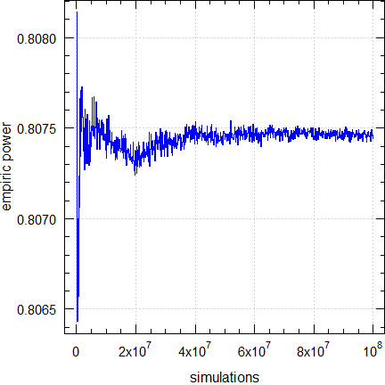
Fig. 2 Empiric power for CV = 0.25, n = 28.
In the Monte Carlo method values approach the exact one asymptotically.
Q: Why give links to some references an HTTP-error 404 ‘Not found’?
A: I checked all URLs in March 2025. Contrary to us mere mortals who have to maintain a version control of documents, agencies don’t care. They change the structure of their websites, don’t establish automatic redirects, rename or even delete files… Quod licet Iovi, non licet bovi
If you discover an error, please drop me a note at [email protected]..Q: I still have questions. How to proceed?
A: The preferred method is to register at the BEBA Forum and post your question in the category (please read the Forum’s Policy first).
You can contact me at [email protected]. Be warned – I will charge you for anything beyond most basic questions.
top of section ↩︎ previous section ↩︎
Licenses
 Helmut Schütz 2025
![]() ,
,
PowerTOST, arsenal, and pandoc GPL 3.0;
klippy MIT.
1st version March 10, 2021. Rendered March 7, 2025 12:07 CET
by rmarkdown
via pandoc in 1.09 seconds.
Abbreviations
| Abbreviation | Meaning |
|---|---|
| BE | Bioequivalence |
| \(\small{CV}\) | Coefficient of Variation |
| \(\small{CV_\textrm{inter}}\) | Between-subject Coefficient of Variation |
| \(\small{CV_\textrm{intra}}\) | Within-subject Coefficient of Variation |
| \(\small{H_0}\) | Null hypothesis |
| \(\small{H_1}\) | Alternative hypothesis (also \(\small{H_\textrm{a}}\)) |
| NTID | Narrow Therapeutic Index Drug |
| TOST | Two One-Sided Tests |
| \(\small{\alpha}\) | Nominal level of the test, probability of Type I Error, patient’s risk |
| \(\small{\beta}\) | Probability of Type II Error, producer’s risk |
| \(\small{\pi}\) | Prospective power (\(\small{1-\beta}\)) |
Footnotes and References
Labes D, Schütz H, Lang B. PowerTOST: Power and Sample Size for (Bio)Equivalence Studies. Package version 1.5.6. 2024-03-18. CRAN.↩︎
Heinzen E, Sinnwell J, Atkinson E, Gunderson T, Dougherty G, Votruba P, Lennon R, Hanson A, Goergen K, Lundt E, Broderick B, McCullough M. arsenal: An Arsenal of ‘R’ Functions for Large-Scale Statistical Summaries. Package version 3.6.3. 2021-06-04. CRAN.↩︎
Labes D, Schütz H, Lang B. Package ‘PowerTOST’. March 18, 2024. CRAN.↩︎
Senn S. Guernsey McPearson’s Drug Development Dictionary. April 21, 2020. Online.↩︎
Hoenig JM, Heisey DM. The Abuse of Power: The Pervasive Fallacy of Power Calculations for Data Analysis. Am Stat. 2001; 55(1): 19–24. doi:10.1198/000313001300339897.
 Open
Access.↩︎
Open
Access.↩︎In short: There is no statistical method to ‘correct’ for unequal carryover. It can only be avoided by design, i.e., a sufficiently long washout between periods. According to the guidelines subjects with pre-dose concentrations > 5% of their Cmax can by excluded from the comparison if stated in the protocol.↩︎
Especially important for drugs which are auto-inducers or -inhibitors and biologics.↩︎
Senn S. Statistical Issues in Drug Development. Chichester: John Wiley; 2nd ed 2007.↩︎
Julious SA. Sample Sizes for Clinical Trials. Boca Raton: CRC Press; 2010. Chapter 7.2.↩︎
Common batch release specifications are ±10% of the declared content. Of course, you will try to find a batch of the reference product which is as close as possible to the test (the EMA, the FDA, and the ICH recommend ≤ 5%). However, keep analytical (in)accuracy and (im)precision in mind. Furthermore, the analytical method was only validated for the test. You never can be sure. Try to get a CoA from the originator… Good luck 😉.↩︎
Senn S. Statistical Issues in Drug Development. Chichester: John Wiley; 2004.↩︎
Zhang P. A Simple Formula for Sample Size Calculation in Equivalence Studies. J Biopharm Stat. 2003; 13(3): 529–38. doi:10.1081/BIP-120022772.↩︎
Doyle AC. Adventures of Sherlock Holmes. Adventure I.—A Scandal in Bohemia. The Strand Magazine. 1891; 2(7): 63.↩︎
Schütz H. Sample Size Estimation in Bioequivalence. Evaluation. BEBA Forum. Vienna. 2020-10-23. Online.↩︎
Lenth RV. Two Sample-Size Practices that I Don’t Recommend. October 24, 2000. Online.↩︎
Quoting my late father: »If you believe, go to church.«↩︎
Ring A, Lang B, Kazaroho C, Labes D, Schall R, Schütz H. Sample size determination in bioequivalence studies using statistical assurance. Br J Clin Pharmacol. 2019; 85(10): 2369–77. doi:10.1111/bcp.14055.
Open
Access.↩︎Berger RL, Hsu JC. Bioequivalence Trials, Intersection-Union Tests and Equivalence Confidence Sets. Stat Sci. 1996; 11(4): 283–302. JSTOR:2246021.↩︎
Zeng A. The TOST confidence intervals and the coverage probabilities with R simulation. March 14, 2014. Online.↩︎
With
alpha = 0.5the test effectively reduces to a pass|fail assessment.↩︎The FDA and China’s CDE recommend Reference-Scaled Average Bioequivalence (RSABE) and a comparison of within-subject standard deviations of products – requiring a fully replicated design. It is covered in another article.↩︎
Fieller EC. Some Problems In Interval Estimation. J Royal Stat Soc B. 1954; 16(2): 175–85. JSTOR:2984043.↩︎
Locke CS. An Exact Confidence Interval from Untransformed Data for the Ratio of Two Formulation Means. J Pharmacokin Biopharm. 1984; 12(6): 649–55. doi:10.1007/bf01059558.↩︎
EMEA, CPMP. Points to Consider on Switching between Superiority and Non-Inferiority. London. 27 July 2000. Online.↩︎
Owen DB. A special case of a bivariate non-central t-distribution. Biometrika. 1965; 52(3/4): 437–46. doi:10.2307/2333696.↩︎
Zheng C, Wang J, Zhao L. Testing bioequivalence for multiple formulations with power and sample size calculations. Pharm Stat. 2012; 11(4): 334–41. doi:10.1002/pst.1522.↩︎
Hauschke D, Steinijans VW, Pigeot I. Bioequivalence Studies in Drug Development. Chichester: John Wiley; 2007. Tables 5.1–5.3.↩︎
Chow SC, Liu J-p. Design and Analysis of Bioavailability and Bioequivalence Studies. Boca Raton: CRC Press; 3rd ed. 2009. Table 5.4.1.↩︎
Diletti E, Hauschke D, Steinijans VW. Sample size determination for bioequivalence assessment by means of confidence intervals. Int J Clin Pharmacol Ther Toxicol. 1991; 29(1): 1–8. PMID 2004861.↩︎
Diletti E, Hauschke D, Steinijans VW. Sample size determination: Extended tables for the multiplicative model and bioequivalence ranges of 0.9 to 1.11 and 0.7 to 1.43. Int J Clin Pharmacol Ther Toxicol. 1992; 30(Suppl.1): S59–62. PMID 1601533.↩︎
Jackson AJ (ed.). Generics and Bioequvalence. Boca Raton: Taylor & Francis / CRC Press; 1994 (reissued 2019). p. 21.↩︎
Phillips KM. Power of the Two One-Sided Tests Procedure in Bioequivalence. J Pharmacokin Biopharm. 1990; 18(2): 137–44. doi:10.1007/BF01063556. Table I.↩︎
The R Foundation for Statistical Computing. A Guidance Document for the Use of R in Regulated Clinical Trial Environments. Vienna. October 18, 2021. Online.↩︎
The R Foundation for Statistical Computing. R: Software Development Life Cycle. A Description of R’s Development, Testing, Release and Maintenance Processes. Vienna. October 18, 2021. Online.↩︎
FDA. General Principles of Software Validation; Final Guidance for Industry and FDA Staff. Rockville. January 11, 2002. Download.↩︎
FDA. Statistical Software Clarifying Statement. May 6, 2015. Online.↩︎
WHO. Guidance for organizations performing in vivo bioequivalence studies. Technical Report Series No. 996, Annex 9. Section 4. Geneva. May 2016. Online.↩︎
EMA, GCP IWG. Guideline on computerised systems and electronic data in clinical trials. Amsterdam. 9 March 2023. Online.↩︎