Consider allowing JavaScript. Otherwise, you have to be proficient in reading LaTeX since formulas will not be rendered. Furthermore, the table of contents in the left column for navigation will not be available and code-folding not supported. Sorry for the inconvenience.

Examples in this article were generated with 4.3.3 by the packages TeachingDemos,¹ magicaxis,² PowerTOST,³ Power2Stage,⁴ nlme,⁵ lme4,⁶ and lmerTest.⁷

The right-hand badges give the respective section’s ‘level’.

Basics about maths and/or sample size methodology – requiring no or only limited statistical expertise.

These sections are the most important ones. They are – hopefully – easily comprehensible even for novices.

A somewhat higher knowledge of statistics and/or R is required. May be skipped or reserved for a later reading.

An advanced knowledge of statistics and/or R is required. Not recommended for beginners in particular.

If you are not a neRd or statistics afficionado, skipping is recommended. Suggested for experts but might be confusing for others.

Click to show / hide R code.
To copy R code to the clipboard click on the icon in the top left corner.

Abbreviation	Meaning
ABE	Average Bioequivalence
ABEL	Average Bioequivalence with Expanding Limits
$\small{CV}$ ($\small{CV_\text{wT}}$, $\small{CV_\text{wR}}$)	Within-subject Coefficient of Variation (of the Test and Reference treatment)
GMR	Geometric Mean Ratio
HVD(P)	Highly Variable Drug (Product)
RSABE	Reference-scaled Average Bioequivalence
SABE	Scaled Average Bioequivalence
$\small{s_\text{wR}}$	Within-subject standard devtaion of the Reference treatment
TOST	Two One-Sided Tests

Introduction

What are simulations and why may we need them?

In statistics (or better, in science in general) we prefer to obtain results by an analytical calculation. Remember your classes in algebra and calculus? That’s the stuff.
However, sometimes the desire for an ‘exact’ solution of a problem reminds on the hunt for unobtainium.

If you know the movie Hidden Figures maybe you recall the scene where Katherine Johnson solved the transition from the elliptic orbit of the Mercury capsule to the parabolic re-entry trajectory by Euler’s approximations. Given, not a simulation but a numerical method since an algebraic solution simply did not – and will never – exist.

Least-squares and maximum-likelihood optimizations are part of our bread-and-butter jobs. Nobody complains that the result is not ‘exact’.

“Statistics. A sort of elementary form of mathematics which consists of adding things together and occasionally squaring them.

Stephen Senn

However, sometimes numerical methods are not feasible if the problem gets too large. Large in this context means many parameters, a high number of data points to fit, or both.
Two examples:

Wheather forecasting or – even worse – climate modeling.
In principle all we need is known for a long time: The Navier–Stokes equations, the van der Waals equation, the first law of thermodynamics, the continuity equation, and the equation of radiative transfer. Great. Unfortunatelly, combining them results in coupled partial differential equations. Can we solve them for any given state of the atmosphere? Nope.
BTW, 42 is not the correct answer.
The only way out are numerical models run on – really – large numbercrunchers.

The n-body problem. If you are in science fiction novels, I recommend The Three-Body Problem by Liu Cixin. Analytical solutions for more than two bodies don’t exist.

Fig. 1 Three body problem.

Approximate trajectories of three identical bodies located at the vertices of a scalene triangle and having zero initial velocities. It is seen that the center of mass, in accordance with the law of conservation of momentum, remains in place.
© Dnttllthmmnm @ wikimedia commons

How many objects are in the solar system? You name it. Nevertheless, after a 9½ years and a five billion km journey the New Horizons space probe had a 12,472 km close encounter with Pluto.
THX to numerics & simulations.

When it comes to (bio)equivalence, we need simulations in various areas. One is power calculation / sample size estimation for Scaled Average Bioequivalence and the other for adaptive sequential Two-Stage Designs for parallel groups.

“Whenever a theory appears to you as the only possible one, take this as a sign that you have neither understood the theory nor the problem which it was intended to solve.
Karl R. Popper

As we will see in the examples, in the Monte Carlo method values approach the exact one asymptotically.

top of section ↩︎

Examples

# attach libraries to run the examples
library(TeachingDemos)
library(magicaxis)
library(PowerTOST)
library(Power2Stage)
library(nlme)
library(lmerTest)

All scripts were run on a Xeon E3-1245v3 @ 3.40GHz (1/4 cores) 16GB RAM with R 4.3.3 on Windows 7 build 7601, Service Pack 1, Universal C Runtime 10.0.10240.16390

Rolling two dice

Here it’s easy to get the average sum of pips. If you remember probability and combinatorics, you will get the answer seven. If you are a gambler, you simply know it. If you have two at hand, roll them. Of course, you will get anything between the possible extremes (two and twelve) in a single roll. But you would need many rolls to come close to the theoretical average seven. Since this is a boring excercise (unless you find an idiot betting against seven), let R do the job (one to ten thousand rolls):

set.seed(123)
nsims <- ceiling(10^(seq(0, 4, 0.01)))
df    <- data.frame(nsims = nsims, sum.pips = NA)
for (i in seq_along(nsims)) {
  df[i, 2] <- sum(dice(rolls = nsims[i],
                       ndice = 2, sides = 6))/nsims[i]
}
ylim <- c(2, 12)
j    <- 10^(seq(0, 4, 1))
mean.j <- numeric()
for (i in seq_along(j)) {
  mean.j[i] <- mean(df[df$nsims == j[i], 2])
}
dev.new(width = 4.5, height = 4.5)
op <- par(no.readonly = TRUE)
par(mar = c(3, 3, 3, 0.1), cex.axis = 0.9,
    mgp = c(2, 0.5, 0))
plot(df$nsims, df[, 1], type = "n",
     ylim = ylim, axes = FALSE, log = "x",
     xlab = "Number of simulated rolls",
     ylab = "Average sum of pips")
mtext("Average at 1, 10, \u2026", 3, line = 2)
grid(); box()
abline(h = 7)
magaxis(1)
magaxis(2, minorn = 2, las = 1)
axis(3, labels = sprintf("%.2f", mean.j), at = j)
points(df$nsims, df[, 2], pch = 21,
       col = "blue", bg = "#9090FF80", cex = 1.15)
par(op)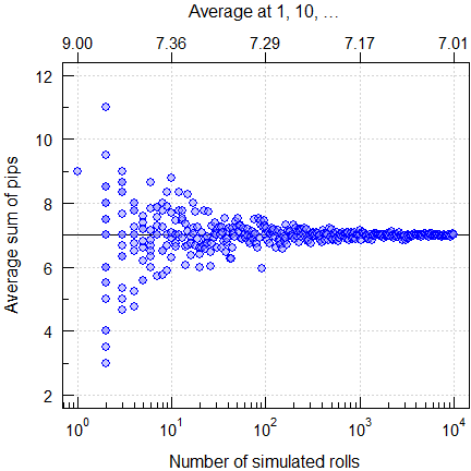

Fig. 2 Rolling two dice.

top of section ↩︎ previous section ↩︎

Estimating π

We generate a set of uniformly distributed coordinates $\small{\left\{x|y\right\}}$ in the range $\small{\left\{-1|+1\right\}}$.
According to Mr. Pythagoras all $\small{x^2+y^2\leq1}$ are at or within the unit circle and coded in blue. Since $\small{A=\frac{\pi\,d^2}{4}}$ and $\small{d=1}$, we get an estimate of $\small{\pi}$ by 4 times the number of coded points (the ‘area’) divided by the number of simulations. Here for fifty thousand:

set.seed(12345678)
nsims <- 5e4
x <- runif(nsims, -1, 1)
y <- runif(nsims, -1, 1)
is.inside   <- (x^2 + y^2) <= 1
pi.estimate <- 4 * sum(is.inside) / nsims
dev.new(width = 5.7, height = 5.7)
op <- par(no.readonly = TRUE)
par(pty = "s", cex.axis = 0.9, mgp = c(2, 0.5, 0))
main <- bquote(italic(pi)*-estimate == .(pi.estimate))
plot(c(-1, 1), c(-1, 1), type = "n", axes = FALSE,
     xlim = c(-1, 1), ylim = c(-1, 1), font.main = 1,
     xlab = expression(italic(x)),
     ylab = expression(italic(y)), cex.main = 1.1,
     main = main)
points(x[is.inside], y[is.inside], pch = '.', 
       col = "blue")
points(x[!is.inside], y[!is.inside], pch = '.',
       col = "lightgrey")
magaxis(1:2, las = 1)
abline(h = 0, v = 0)
box()
par(op)

Fig. 3 Estimating $\small{\pi}$ (unit circle inclusion method).

This was a lucky punch since the convergence is lousy. To get a stable estimate with just four correct significant digits, we need at least one hundred million (‼) simulations.

Another slowly converging approach is simulating Buffon’s needle.⁸

# Cave: Extremely long runtime
set.seed(123456)
buffon_needles <- function(l, n = 1) {
  H <- rep(0, n)
  for (i in 1:n) {
    M  <- runif(2)
    D  <- c(1, 1)
    while (norm(D, type = '2') > 1) {
      D <- runif(2)
    }
    DD   <- D/norm(D, type = '2')
    E1   <- M + l / 2 * DD
    E2   <- M - l / 2 * DD
    H[i] <- (E1[1] < 0) |
            (E1[1] > 1) |
            (E2[1] < 0) |
            (E2[1] > 1)
  }
  return(H)
}
l     <- 0.4
nsims <- as.integer(10^(seq(3, 7, 0.05)))
pb    <- txtProgressBar(0, 1, 0, width = NA, style = 3)
for (i in 1:nrow(df)) {
  HHH <- buffon_needles(l, n = df$nsims[i])
  df$pi.estimate[i] <- 2 * l / mean(HHH)
  setTxtProgressBar(pb, i/nrow(df))
}
close(pb)
tail(df, 1) # show last
dev.new(width = 4.5, height = 4.5)
op <- par(no.readonly = TRUE)
par(mar = c(3, 3, 0, 0), cex.axis = 0.9,
    mgp = c(2, 0.5, 0))
plot(df$nsims, df$pi.estimate, type = "n",
     log = "x", axes = FALSE,
     xlab = "Number of simulations",
     ylab = expression(italic(pi)*"-estimate"))
grid(); box()
abline(h = pi, col = "red")
magaxis(1:2, las = 1)
points(df$nsims, df$pi.estimate, pch = 21,
       col = "blue", bg = "#9090FF80", cex = 1.15)
par(op)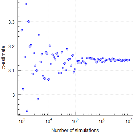

Fig. 4 Estimating $\small{\pi}$ (Buffon’s needle drops).

Of course, there are extremely efficient methods like the Chudnovsky algorithm (with March 2024 the record holder with one 105 trillion digits).

q      <- 0:1L
pi.rep <- 0
for (i in seq_along(q)) {
  pi.rep <- pi.rep - 
            12/640320^(3/2) *
            (factorial(6 * q[i]) * (13591409 + 545140134 *q[i])) /
            (factorial(3 * q[i]) * factorial(q[i])^3 *
             -640320^(3 * q[i]))
}
pi.approx <- 1/pi.rep
comp <- data.frame(q = as.integer(max(q)),
                   pi = sprintf("%.15f", pi),
                   pi.approx = sprintf("%.15f", pi.approx),
                   RE = sprintf("%-.15f%%",
                               100 * (pi.approx - pi) / pi))
print(comp, row.names = FALSE)

#  q                pi         pi.approx                  RE
#  1 3.141592653589793 3.141592653589675 -0.000000000003746%

Note that increasing the number of iterations q does not improve the result. Since this is an extremely efficient algorithm, we are already at the numeric resolution of a 64 bit numeric, which is ~2.220446·10^-16.

The wonderland of representing numbers on digital computers is elaborated in another article.

top of section ↩︎ previous example ↩︎ previous section ↩︎

LLOQ

A bioanalytical method should have a sufficiently low Limit of Quantification in order to assess potential carryover (subjects with pre-dose concentrations of $\small{\gt 5\%\:C_\textrm{max}}$ can be excluded from the comparison) and avoid a large extrapolated $\small{AUC}$.

Say, we have a bioanalytical method with $\small{\textrm{LLOQ}=5\%\:C_\textrm{max}}$ and a $\small{CV}$ at the LLOQ of 20%. Note, that this has nothing to do with the maximum acceptable $\small{CV}$ of 15% in method validation (calibrators, quality control samples). The variability in pre-dose samples might well be higher.
What is the probability to find subjects with pre-dose concentrations $\small{\gt\textrm{LLOQ}}$?

set.seed(123456)
Cmax     <- setNames(c(100, 0.2), c("mu", "CV"))
pct.Cmax <- 5
LLOQ     <- pct.Cmax * Cmax[["mu"]] / 100
nsims    <- c(1e2, 5e2, 1e3, 5e3, 1e4, 5e4, 1e5)
exact    <- plnorm(LLOQ, mean = log(LLOQ) - 0.5 * log(Cmax[["CV"]]^2 + 1),
                         sd   = sqrt(log(Cmax[["CV"]]^2 + 1)),
                   lower.tail = FALSE)
df    <- data.frame(simulations = nsims,
                    exact = rep(exact, length(nsims)),
                    simulated = NA, SE = NA, RE = NA)
for (i in 1:nrow(df)) {
  pre.dose        <- rlnorm(n       = nsims[i],
                            meanlog = log(Cmax[["mu"]]) -
                                      0.5 * log(Cmax[["CV"]]^2 + 1),
                            sdlog   = sqrt(log(Cmax[["CV"]]^2 + 1))) *
                     pct.Cmax / 100
  df$simulated[i] <- signif(sum(pre.dose > LLOQ) / nsims[i], 4)
  df$SE[i]        <- signif(sqrt(0.025 / i), 4)
  df$RE           <- 100 * (df$simulated - exact) / exact
}
df$exact       <- signif(df$exact, 4)
df$RE          <- sprintf("%+.4f%%", df$RE)
df$simulations <- formatC(df$simulations, format = "f",
                          digits = 0, big.mark=",")
names(df)[c(1, 3)] <- c("sim\u2019s", "sim\u2019d")
print(df, row.names = FALSE)

#    sim’s  exact  sim’d      SE       RE
#      100 0.4606 0.4500 0.15810 -2.2930%
#      500 0.4606 0.5040 0.11180 +9.4318%
#    1,000 0.4606 0.4620 0.09129 +0.3125%
#    5,000 0.4606 0.4642 0.07906 +0.7902%
#   10,000 0.4606 0.4647 0.07071 +0.8987%
#   50,000 0.4606 0.4617 0.06455 +0.2474%
#  100,000 0.4606 0.4624 0.05976 +0.3993%

That’s surprisingly high, right? If you have twenty-four subjects in the study, you can expect at least eleven with pre-dose concentrations above the LLOQ. Hence, aim lower.

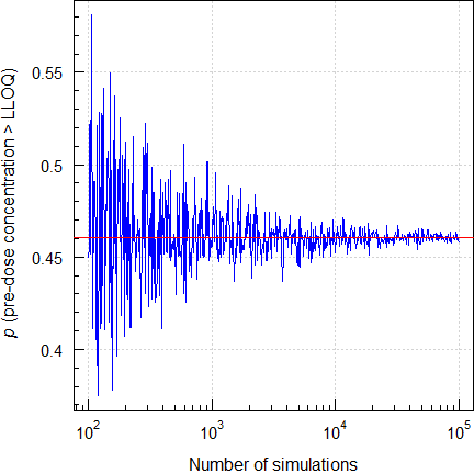
Fig. 5 Simulating pre-dose concentrations $\small{\gt\textrm{LLOQ}}$.

Furthermore, the probability depends on the variability. This time only the exact results.

CV       <- c(0.2, 0.4)
Cmax     <- setNames(c(100, CV[1]), c("mu", "CV"))
limit    <- 5 * Cmax[["mu"]] / 100
pct.Cmax <- 5L:2L
LLOQ     <- pct.Cmax * Cmax[["mu"]] / 100
df1      <- data.frame(Cmax = rep(Cmax[["mu"]], length(LLOQ)),
                       CV = Cmax[["CV"]],  LLOQ = LLOQ, p = NA_real_)
for (i in 1:nrow(df1)) {
  df1$p[i] <- plnorm(limit,
                     mean = log(df1$LLOQ[i]) - 0.5 * log(Cmax[["CV"]]^2 + 1),
                     sd   = sqrt(log(Cmax[["CV"]]^2 + 1)),
                     lower.tail = FALSE)
}
Cmax     <- setNames(c(100, CV[2]), c("mu", "CV"))
df2      <- data.frame(Cmax = rep(Cmax[["mu"]], length(LLOQ)),
                       CV = Cmax[["CV"]],  LLOQ = LLOQ, p = NA_real_)
for (i in 1:nrow(df2)) {
  df2$p[i] <- plnorm(limit,
                     mean = log(df2$LLOQ[i]) - 0.5 * log(Cmax[["CV"]]^2 + 1),
                     sd   = sqrt(log(Cmax[["CV"]]^2 + 1)),
                     lower.tail = FALSE)
}
df <- rbind(df1, df2)
df$p <- sprintf("%.5f%%", 100 * df$p)
names(df)[4] <- "pre-dose > LLOQ"
print(df, row.names = FALSE)

#  Cmax  CV LLOQ pre-dose > LLOQ
#   100 0.2    5       46.05608%
#   100 0.2    4       11.01429%
#   100 0.2    3        0.36988%
#   100 0.2    2        0.00011%
#   100 0.4    5       42.36257%
#   100 0.4    4       22.01048%
#   100 0.4    3        6.44348%
#   100 0.4    2        0.50697%

If the $\small{CV}$ is 20%, an LLOQ of 3% of $\small{C_\textrm{max}}$ is sufficient. However, if it is 40%, it’s better to aim at ≤ 2% of $\small{C_\textrm{max}}$.

top of section ↩︎ previous example ↩︎ previous section ↩︎

TOST and its relatives

Power

Over the top, since an exact (analytical) solution exists. However, if you don’t trust in it, simulations are possible with the function power.TOST.sim(), employing the distributional properties ($\small{\sigma^2}$ follows a $\small{\chi^2\textrm{-}}$distribution with $\small{n-2}$ degrees of freedom and $\small{\log_{e}(\theta_0)}$ follows a normal distribution).⁹

Empiric power, its standard error, its relative error compared to the exact power, and execution times:

CV    <- 0.25
n     <- sampleN.TOST(CV = CV,
                      print = FALSE)[["Sample size"]]
nsims <- c(1e5L, 5e5L, 1e6L, 5e6L,1e7L, 5e7L, 1e8L)
exact <- power.TOST(CV = CV, n = n)
x     <- data.frame(sims = nsims,
                    exact = rep(exact, length(nsims)),
                    sim = NA_real_, SE = NA_real_,
                    RE = NA_real_)
for (i in seq_along(nsims)) {
  st        <- proc.time()[[3]]
  x$sim[i]  <- power.TOST.sim(CV = CV, n = n,
                              nsims = nsims[i])
  x$secs[i] <- proc.time()[[3]] - st
  x$SE[i]   <- sqrt(0.5 * x$sim[i] / nsims[i])
}
x$RE    <- 100 * (x$sim - exact) / exact
x$exact <- signif(x$exact, 5)
x$SE    <- round(x$SE, 6)
x$RE    <- sprintf("%+.4f%%", x$RE)
x$sim   <- signif(x$sim, 5)
x$sims  <- prettyNum(x$sims, format = "i", big.mark = ",")
names(x)[c(1, 3)] <- c("sim\u2019s", "sim\u2019d")
print(x, row.names = FALSE)

#        sim’s   exact   sim’d       SE       RE   secs
#      100,000 0.80744 0.80814 0.002010 +0.0868%   0.15
#      500,000 0.80744 0.80699 0.000898 -0.0552%   0.81
#    1,000,000 0.80744 0.80766 0.000635 +0.0279%   1.61
#    5,000,000 0.80744 0.80751 0.000284 +0.0090%   8.08
#   10,000,000 0.80744 0.80733 0.000201 -0.0136%  16.13
#   50,000,000 0.80744 0.80743 0.000090 -0.0009%  81.62
#  100,000,000 0.80744 0.80744 0.000064 +0.0001% 162.01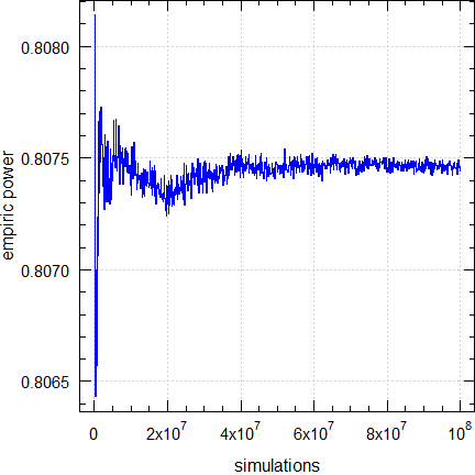

Fig. 6 Empiric power of TOST (2×2×2 crossover, T/R ratio 0.95, n 28).

The convergence is good. Even with only 10,000 simulations the relative error would be < 0.3%.

top of section ↩︎ previous example ↩︎ previous section ↩︎

Type I Error

We know that $\small{\alpha}$ (the probability of the Type I Error) in the TOST procedure and the operationally equivalent confidence interval inclusion approach never exceeds the nominal level (generally 0.05). In e.g., a 2×2×2 crossover design with CV 25% and 28 subjects $\small{\alpha\simeq 0.04999963\ldots}$
We can simulate a large number of studies with a T/R-ratio at one of the borders of the acceptance range and assess them for ABE as well, i.e., assume that the null hypothesis is true. We expect ≤ 5% of studies to pass. The number of passing studies divided by the number of simulations gives the empiric Type I Error.

# Cave: Long run-time!
runs  <- 5
nsims <- as.integer(10^(seq(3, 7, 0.1)))
df    <- data.frame(run = 1:runs,
                    nsims = rep(nsims, each = runs),
                    binomial.lower = NA_real_,
                    binomial.upper = NA_real_,
                    TIE = NA_real_)
CV    <- 0.25
n     <- sampleN.TOST(CV = CV,
                      print = FALSE)[["Sample size"]]
exact <- power.TOST(theta0 = 1.25, CV = CV, n = n)
pb    <- txtProgressBar(0, 1, 0, width = NA, style = 3)
for (i in 1:nrow(df)) {
  x   <- ceiling(0.05 * df$nsims[i])
  b.t <- binom.test(x, df$nsims[i], alternative =
                    "two.sided")[["conf.int"]]
  df[i, 3:4] <- as.numeric(b.t)
  ifelse (df$run[i] == 1,
    setseed <- TRUE,
    setseed <- FALSE)
  df$TIE[i] <- power.TOST.sim(theta0 = 1.25, CV = CV,
                              n = n, nsims = df$nsims[i],
                              setseed = setseed)
  setTxtProgressBar(pb, i / nrow(df))
}
close(pb)
ylim <- range(df[, 3:5])
dev.new(width = 4.5, height = 4.5)
op <- par(no.readonly = TRUE)
par(mar = c(3, 3.5, 0, 0), cex.axis = 0.9,
    mgp = c(2, 0.5, 0))
plot(df$nsims, df[, 2], type = "n", log = "x",
     ylim = ylim, axes = FALSE,
     xlab = "Number of simulations", ylab = "")
mtext("Empiric Type I Error", 2, line = 2.5)
grid(); box()
abline(h = exact, col = "red")
lines(df$nsims, df[, 3])
lines(df$nsims, df[, 4])
magaxis(1:2, las = 1)
for (i in 1:nrow(df)) {
  ifelse (df$run[i] == 1, pch <- 19, pch <- 1)
  points(df$nsims[i], df$TIE[i], pch = pch,
         col = "blue", cex = 1.15)
}
par(op)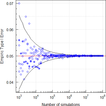

Fig. 7 Empiric Type I Error of TOST (2×2×2 crossover, CV 0.25, T/R ratio 0.95, n 28).

Five repeated runs. The filled circles are runs with a fixed seed of 123456 and open circles ones with random seeds. The lines show the upper and lower significance limits of the binomial test. We see that convergence of this problem is poor.

However, since all variants SABE and adaptive Two-Stage Designs are frameworks, exact methods don’t exist. We have to leave our comfort zone and resort to – reasonably large – simulations. Therefore, in e.g., assessing a potentially inflated Type I Error 10⁶ simulations are common nowadays.

# Cave: Long run-time!
runs  <- 5
nsims <- as.integer(10^(seq(3, 7, 0.1)))
df    <- data.frame(run = 1:runs,
                    nsims = rep(nsims, each = runs),
                    binomial = NA_real_,
                    TIE = NA_real_)
CVwR  <- 0.30
n     <- sampleN.scABEL(CV = CVwR, design = "2x2x4",
                        details = FALSE,
                        print = FALSE)[["Sample size"]]
pb    <- txtProgressBar(0, 1, 0, width = NA, style = 3)
for (i in 1:nrow(df)) {
  x        <- ceiling(0.05 * df$nsims[i])
  df[i, 3] <- binom.test(x, df$nsims[i],
                        alternative = "less")[["conf.int"]][2]
  ifelse (df$run[i] == 1,
    setseed <- TRUE,
    setseed <- FALSE)
  df$TIE[i] <- power.scABEL(CV = CVwR, design = "2x2x4",
                            theta0 = 1.25, n = n,
                            nsims = df$nsims[i],
                            setseed = setseed)
  setTxtProgressBar(pb, i / nrow(df))
}
close(pb)
dev.new(width = 4.5, height = 4.5)
op   <- par(no.readonly = TRUE)
par(mar = c(3, 3.5, 0, 0), cex.axis = 0.9,
    mgp = c(2, 0.5, 0))
plot(df$nsims, df[, 2], type = "n", log = "x",
     ylim = range(df[, 3:4]), axes = FALSE,
     xlab = "Number of simulations", ylab = "")
mtext("Empiric Type I Error", 2, line = 2.5)
grid()
abline(h = 0.05, col = "red")
box()
lines(df$nsims, df[, 3])
magaxis(1:2, las = 1)
for (i in 1:nrow(df)) {
  ifelse (df$run[i] == 1, pch <- 19, pch <- 1)
  points(df$nsims[i], df$TIE[i], pch = pch,
         col = "blue", cex = 1.15)
}
par(op)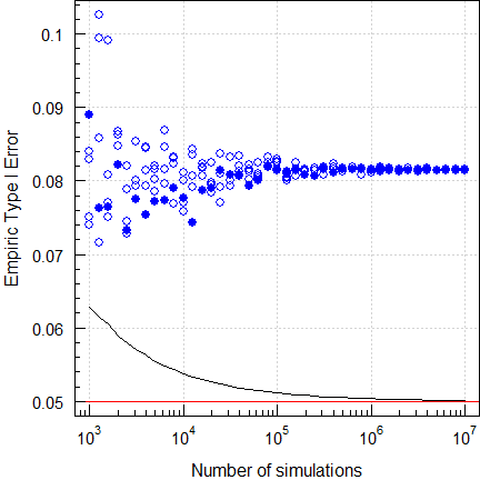

Fig. 8 Empiric Type I Error of ABEL (2-sequence 4-period full replicate design, CV_wR = CV_wT 30%, n 34).

Five repeated runs again. We see that the Type I Error is inflated. Although obvious already with a small number of simulations (all results lie above the significance limit of the binomal test), a higher number of simulations is recommended for a stable result.

# Cave: Long run-time!
runs  <- 5
nsims <- as.integer(10^(seq(3, 7, 0.1)))
df    <- data.frame(run = 1:runs,
                    nsims = rep(nsims, each = runs),
                    binomial = NA_real_,
                    TIE = NA_real_)
CVwR  <- 0.30
n     <- sampleN.RSABE(CV = CVwR, design = "2x2x4",
                       details = FALSE,
                       print = FALSE)[["Sample size"]]
pb    <- txtProgressBar(0, 1, 0, width = NA, style = 3)
for (i in 1:nrow(df)) {
  x        <- ceiling(0.05 * df$nsims[i])
  df[i, 3] <- binom.test(x, df$nsims[i],
                        alternative = "less")[["conf.int"]][2]
  ifelse (df$run[i] == 1,
    setseed <- TRUE,
    setseed <- FALSE)
  df$TIE[i] <- power.RSABE(CV = CVwR, design = "2x2x4",
                           theta0 = 1.25, n = n,
                           nsims = df$nsims[i],
                           setseed = setseed)
  setTxtProgressBar(pb, i/nrow(df))
}
close(pb)
dev.new(width = 4.5, height = 4.5)
op   <- par(no.readonly = TRUE)
par(mar = c(3, 3.5, 0, 0), cex.axis = 0.9,
    mgp = c(2, 0.5, 0))
plot(df$nsims, df[, 2], type = "n", log = "x",
     ylim = range(df[, 3:4]), axes = FALSE,
     xlab = "Number of simulations", ylab = "")
mtext("Empiric Type I Error", 2, line = 2.5)
grid()
abline(h = 0.05, col = "red")
box()
lines(df$nsims, df[, 3])
magaxis(1:2, las = 1)
for (i in 1:nrow(df)) {
  ifelse (df$run[i] == 1, pch <- 19, pch <- 1)
  points(df$nsims[i], df$TIE[i], pch = pch,
         col = "blue", cex = 1.15)
}
par(op)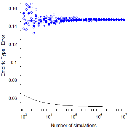

Fig. 9 Empiric Type I Error of RSABE (2-sequence 4-period full replicate design, CV_wR = CV_wT 30%, n 32).

A picture tells more than a thousand words…

Let’s explore a ‘Type 1’ adaptive two-stage design¹⁰ with $\small{\alpha_\text{adj}=0.0294}$ (Method B¹¹) at the reported location of the maximum Type I Error.

# Cave: Extremely long run-time!
runs  <- 5
nsims <- as.integer(10^(seq(3, 7, 0.1)))
df    <- data.frame(run = 1:runs,
                    nsims = rep(nsims, each = runs),
                    binomial = NA_real_,
                    TIE = NA_real_)
CV    <- 0.20
n1    <- 12
pb    <- txtProgressBar(0, 1, 0, width = NA, style = 3)
for (i in 1:nrow(df)) {
  x         <- ceiling(0.05 * df$nsims[i])
  df[i, 3]  <- binom.test(x, df$nsims[i],
                        alternative = "less")[["conf.int"]][2]
  ifelse (df$run[i] == 1,
    setseed <- TRUE,
    setseed <- FALSE)
  df$TIE[i] <- power.tsd(CV = CV, n1 = n1,
                         theta0 = 1.25,
                         nsims = df$nsims[i],
                         setseed = setseed)$pBE
  setTxtProgressBar(pb, i / nrow(df))
}
close(pb)
dev.new(width = 4.5, height = 4.5)
op   <- par(no.readonly = TRUE)
par(mar = c(3, 3.5, 0, 0), cex.axis = 0.9,
    mgp = c(2, 0.5, 0))
plot(df$nsims, df[, 2], type = "n", log = "x",
     ylim = range(df[, 3:4]), axes = FALSE,
     xlab = "Number of simulations", ylab = "")
mtext("Empiric Type I Error", 2, line = 2.5)
grid()
abline(h = 0.05, col = "red")
box()
lines(df$nsims, df[, 3])
magaxis(1:2, las = 1)
for (i in 1:nrow(df)) {
  ifelse (df$run[i] == 1, pch <- 19, pch <- 1)
  points(df$nsims[i], df$TIE[i], pch = pch,
         col = "blue", cex = 1.15)
}
par(op)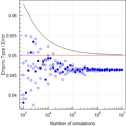

Fig. 10 Empiric Type I Error of a ‘Type 1’ TSD (2×2×2 crossover, CV 0.20, T/R ratio 0.95, n₁ 12).

Although the authors simulated with the simple shifted central t-distribution, we see that the Type I Error is also controlled with a better approximation, the noncentral t-distribution.

top of section ↩︎ previous example ↩︎ previous section ↩︎

Period / sequence effects

Period effects in 2×2×2 crossovers cancel out. The same is true if carryover is equal. If carryover is unequal, the treatment estimate will be biased (see another article for details). Whilst obvious from the statistical model, we can simulate that. Cave: 156 LOC.
If you want to simulate more than 50,000 studies, use the optional argument progress = TRUE in the function call. One million take on my machine a couple of hours to complete and the progress bar gives an idea how many are already finished.

sim.study <- function(CV, CVb, theta0, targetpower,
                      per.effect = c(0, 0),
                      carryover = c(0, 0),
                      nsims, setseed = TRUE,
                      progress = FALSE, # TRUE for a progress bar
                      print = TRUE) {
  if (missing(CV)) stop("CV must be given.")
  if (missing(CVb)) CVb <- CV * 1.5 # arbitrary
  if (missing(theta0)) stop("theta0 must be given.")
  if (length(per.effect) == 1) per.effect <- c(0, per.effect)
  if (missing(targetpower)) stop("targetpower must be given.")
  if (missing(nsims)) stop("nsims must be given.")
  if (setseed) set.seed(123456)
  tmp <- sampleN.TOST(CV = CV, theta0 = theta0,
                      targetpower = targetpower,
                      print = FALSE, details = FALSE)
  n    <- tmp[["Sample size"]]
  pwr  <- tmp[["Achieved power"]]
  res  <- data.frame(p = rep(NA_real_, nsims), PE = NA_real_,
                     Bias = NA_real_, lower = NA_real_,
                     upper = NA_real_, BE = FALSE, sig = FALSE)
  sd   <- CV2se(CV)
  sd.b <- CV2se(CVb)
  if (progress) pb <- txtProgressBar(0, 1, 0, width = NA, style = 3)
  for (sim in 1:nsims) {
    subj   <- 1:n
    T      <- rnorm(n = n, mean = log(theta0), sd = sd)
    R      <- rnorm(n = n, mean = 0, sd = sd)
    TR     <- rnorm(n = n, mean = 0, sd = sd.b)
    T      <- T + TR
    R      <- R + TR
    TR.sim <- exp(mean(T) - mean(R))
    data   <- data.frame(subject   = rep(subj, each = 2),
                         period    = 1:2L,
                         sequence  = c(rep("RT", n),
                                       rep("TR", n)),
                         treatment = c(rep(c("R", "T"), n/2),
                                       rep(c("T", "R"), n/2)),
                         logPK     = NA_real_)
    subj.T <- subj.R <- 0L
    for (i in 1:nrow(data)) {
      if (data$treatment[i] == "T") {
        subj.T  <- subj.T + 1L
        if (data$period[i] == 1L) {
          data$logPK[i] <- T[subj.T] + per.effect[1]
      }else {
          data$logPK[i] <- T[subj.T] + per.effect[2] + carryover[1]
        }
    }else {
        subj.R  <- subj.R + 1L
        if (data$period[i] == 1L) {
          data$logPK[i] <- R[subj.R] + per.effect[1]
      }else {
          data$logPK[i] <- R[subj.T] + per.effect[2] + carryover[2]
        }
      }
    }
    cs       <- c("subject", "period", "sequence", "treatment")
    data[cs] <- lapply(data[cs], factor)
    # simple model for speed reasons
    model    <- lm(logPK ~ sequence + subject + period +
                           treatment, data = data)
    PE       <- exp(coef(model)[["treatmentT"]])
    CI       <- exp(confint(model, "treatmentT",
                            level = 1 - 2 * 0.05))
    typeIII  <- anova(model)
    MSdenom  <- typeIII["subject", "Mean Sq"]
    df2      <- typeIII["subject", "Df"]
    fvalue   <- typeIII["sequence", "Mean Sq"] / MSdenom
    df1      <- typeIII["sequence", "Df"]
    typeIII["sequence", 4] <- fvalue
    typeIII["sequence", 5] <- pf(fvalue, df1, df2,
                                 lower.tail = FALSE)
    res[sim, 1:5] <- c(typeIII["sequence", 5], PE,
                     100 * (PE - theta0) / theta0, CI)
    if (round(CI[1], 4) >= 0.80 & round(CI[2], 4) <= 1.25)
      res[sim, 6] <- TRUE
    if (res$p[sim] < 0.1) res$sig[sim] <- TRUE
    if (progress) setTxtProgressBar(pb, sim/nsims)
  }
  if (print) {
    p   <- sum(res$BE) # passed
    f   <- nsims - p   # failed
    txt <- paste("Simulation scenario",
                 "\n  CV               :", sprintf("%7.4f", CV),
                 "\n  theta0           :", sprintf("%7.4f", theta0),
                 "\n  n                :", n,
                 "\n  achieved power   :", sprintf("%7.4f", pwr))
    if (sum(per.effect) == 0) {
      txt <- paste(txt, "\n  no period effects")
  }else {
      txt <- paste(txt, "\n  period effects   :",
                   sprintf("%+.3g,", per.effect[1]),
                   sprintf("%+.3g",  per.effect[2]))
    }
    if (length(unique(carryover)) == 1) {
      if (sum(carryover) == 0) {
        txt <- paste0(txt, ", no carryover")
    }else {
        txt <- paste(txt, "\n  equal carryover  :",
                     sprintf("%+.3g", unique(carryover)))
      }
  }else {
      txt <- paste(txt, "\n  unequal carryover:",
                   sprintf("%+.3g,", carryover[1]),
                   sprintf("%+.3g", carryover[2]))
    }
    txt <- paste(txt,
                 paste0("\n", formatC(nsims, big.mark = ",")),
                 "simulated studies",
                 "\n  Significant sequence effect:",
                  sprintf("%6.2f%%", 100 * sum(res$sig) / nsims),
                  "\n  PE   (median, quartiles)   :",
                  sprintf("%8.4f", median(res$PE)),
                  sprintf("(%.4f, %.4f)",
                  quantile(res$PE, probs = 0.25),
                  quantile(res$PE, probs = 0.75)),
                  "\n  Bias (median, quartiles)   :",
                  sprintf("%+6.2f%%", median(res$Bias)),
                  sprintf("(%+.2f%%, %+.2f%%)",
                  quantile(res$Bias, probs = 0.25),
                  quantile(res$Bias, probs = 0.75)),
                  paste0("\n", formatC(p, big.mark = ",")), "passing studies",
                  sprintf("(empiric power %.4f)", p / nsims),
                  "\n  Significant sequence effect:",
                  sprintf("%6.2f%%", 100 * sum(res$sig[res$BE == TRUE]) / p),
                  "\n  PE   (median, quartiles)   :",
                  sprintf("%8.4f", median(res$PE[res$BE == TRUE])),
                  sprintf("(%.4f, %.4f)",
                  quantile(res$PE[res$BE == TRUE], probs = 0.25),
                  quantile(res$PE[res$BE == TRUE], probs = 0.75)),
                  "\n  Bias (median, quartiles)   :",
                  sprintf("%+6.2f%%", median(res$Bias[res$BE == TRUE])),
                  sprintf("(%+.2f%%, %+.2f%%)",
                  quantile(res$Bias[res$BE == TRUE], probs = 0.25),
                  quantile(res$Bias[res$BE == TRUE], probs = 0.75)),
                  paste0("\n", formatC(f, big.mark = ",")), "failed studies",
                  sprintf("(empiric type II error %.4f)", f / nsims),
                  "\n  Significant sequence effect:",
                  sprintf("%6.2f%%", 100 * sum(res$sig[res$BE == FALSE]) / f),
                  "\n  PE   (median, quartiles)   :",
                  sprintf("%8.4f", median(res$PE[res$BE == FALSE])),
                  sprintf("(%.4f, %.4f)",
                  quantile(res$PE[res$BE == FALSE], probs = 0.25),
                  quantile(res$PE[res$BE == FALSE], probs = 0.75)),
                  "\n  Bias (median, quartiles)   :",
                  sprintf("%+6.2f%%", median(res$Bias[res$BE == FALSE])),
                  sprintf("(%+.2f%%, %+.2f%%)",
                  quantile(res$Bias[res$BE == FALSE], probs = 0.25),
                  quantile(res$Bias[res$BE == FALSE], probs = 0.75)), "\n")
    cat(txt)
  }
  if (progress) close(pb)
  return(res)
  rm(res)
}

Equal carryover

Small period effect (responses in the second period 5% larger than in the first) and large positive – equal – carryover.

res <- sim.study(CV = 0.20, theta0 = 0.95,
                 targetpower = 0.80, per.effect = 0.05,
                 carryover = c(+0.1, +0.1), nsims = 5e4L)

# Simulation scenario 
#   CV               :  0.2000 
#   theta0           :  0.9500 
#   n                : 20 
#   achieved power   :  0.8347 
#   period effects   : +0, +0.05 
#   equal carryover  : +0.1 
# 50,000 simulated studies 
#   Significant sequence effect:  10.03% 
#   PE   (median, quartiles)   :   0.9493 (0.9104, 0.9905) 
#   Bias (median, quartiles)   :  -0.08% (-4.17%, +4.27%) 
# 41,822 passing studies (empiric power 0.8364) 
#   Significant sequence effect:  10.07% 
#   PE   (median, quartiles)   :   0.9609 (0.9297, 0.9980) 
#   Bias (median, quartiles)   :  +1.15% (-2.13%, +5.06%) 
# 8,178 failed studies (empiric type II error 0.1636) 
#   Significant sequence effect:   9.79% 
#   PE   (median, quartiles)   :   0.8720 (0.8519, 0.8883) 
#   Bias (median, quartiles)   :  -8.21% (-10.33%, -6.49%)

As expected: Although there is no true sequence effect, we detect a significant one at approximately the level of test (10%). Hence, we fell into the trap of false positives and such a test is meaningless.

top of section ↩︎ previous example ↩︎ previous section ↩︎

Unequal carryover

Small period effect (responses in the second period 5% larger than in the first) and small unequal carryover of opposite direction.

res <- sim.study(CV = 0.20, theta0 = 0.95,
                 targetpower = 0.80, per.effect = 0.05,
                 carryover = c(+0.02, -0.02), nsims = 5e4L)

# Simulation scenario 
#   CV               :  0.2000 
#   theta0           :  0.9500 
#   n                : 20 
#   achieved power   :  0.8347 
#   period effects   : +0, +0.05 
#   unequal carryover: +0.02, -0.02 
# 50,000 simulated studies 
#   Significant sequence effect:  10.43% 
#   PE   (median, quartiles)   :   0.9684 (0.9288, 1.0106) 
#   Bias (median, quartiles)   :  +1.94% (-2.23%, +6.37%) 
# 44,529 passing studies (empiric power 0.8906) 
#   Significant sequence effect:  10.50% 
#   PE   (median, quartiles)   :   0.9749 (0.9409, 1.0136) 
#   Bias (median, quartiles)   :  +2.62% (-0.96%, +6.69%) 
# 5,471 failed studies (empiric type II error 0.1094) 
#   Significant sequence effect:   9.87% 
#   PE   (median, quartiles)   :   0.8782 (0.8590, 0.8972) 
#   Bias (median, quartiles)   :  -7.56% (-9.58%, -5.56%)

Although there is a true unequal carryover, the percentage of studies where it is detected is not substantially above the false positive rate. On the average – due to the unequal carryover – the Test treatment is ‘pushed up’ in the second period and the Reference treatment ‘pulled down’. That is also reflected in the empiric power (~89%) which is larger than expected (~83%).
A bias can only be avoided by design (i.e., a sufficiently long washout).

top of section ↩︎ previous example ↩︎ previous section ↩︎

Sample size for SABE

Since the implemented methods for Scaled Average Bioequivalence are frameworks (decision schemes), where the degree of scaling depends on the realized (observed) variability of the reference, an exact method for power and hence, the sample size does not exist. Therefore, simulations are required. For details see the articles about Average Bioquivalence with Expanding Limits (ABEL) and Reference-scaled Average Bioquivalence (RSABE).

In the following comparisons to the tables of Tóthfalusi and Endrényi.¹²

ABEL

Table A2¹² gives for a 4-period full replicate study (the EMA’s method), GMR 0.85, CV_wR 50%, and ≥ 80% power a sample size of 54 (10,000 simulations; filled red circle), whilst the function sampleN.scABEL() of PowerTOST gives only 52 (with its default of 100,000 simulations; filled green circle).

runs  <- 5
nsims <- as.integer(10^(seq(3, 6, 0.1)))
df    <- data.frame(run = 1:runs,
                    nsims = rep(nsims, each = runs),
                    n = NA)
pb    <- txtProgressBar(0, 1, 0, width = NA, style = 3)
for (i in 1:nrow(df)) {
    ifelse (df$run[i] == 1,
      setseed <- TRUE,
      setseed <- FALSE)
    df$n[i] <- sampleN.scABEL(theta0 = 0.85, CV = 0.5,
                              nsims = df$nsims[i],
                              setseed = setseed,
                              design = "2x2x4",
                              targetpower = 0.8,
                              print = FALSE,
                              details = FALSE)[["Sample size"]]
  setTxtProgressBar(pb, i/nrow(df))
}
close(pb)
ylim <- range(df$n)
dev.new(width = 4.5, height = 4.5)
op <- par(no.readonly = TRUE)
par(mar = c(3, 3, 0, 0), cex.axis = 0.9,
    mgp = c(2, 0.5, 0))
plot(df$nsims, df$n, type = "n", log = "x", ylim = ylim,
     axes = FALSE, xlab = "Number of simulations",
     ylab = "Sample size")
grid(); box()
magaxis(1)
magaxis(2, minorn = 2, las = 1)
for (i in 1:nrow(df)) {
  ifelse (df$run[i] == 1, pch <- 19, pch <- 1)
  points(df$nsims[i], df$n[i], pch = pch,
         col = "blue", cex = 1.15)
}
points(1e5, 52, pch = 16, col = "#00AA00", cex = 1.15)
points(1e4, 54, pch = 16, col = "red", cex = 1.15)
par(op)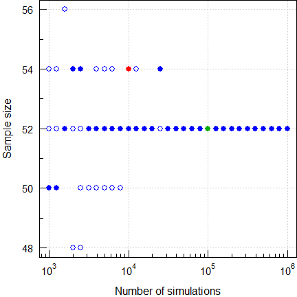

Fig. 11 Sample size for ABEL (2×2×4 replicate, CV 0.50, GMR 0.85, power ≥0.80).

Five runs. Filled circles are with a fixed seed of 123456 and open circles with random seeds. With only 10,000 simulations I got¹³ four times 50, once 52, and once 54 (like ‘The Two Lászlós’). If you have more runs, you will get in some of them more extreme ones (in 1,000 runs of 10,000 I got a median of 52 and a range of 48–56). This wide range demonstrates that the result is not stable yet. Hence, we need at least 50,000 simulations to arrive at 52 as a stable result. Although you are free to opt for more than the default of 100,000, it’s a waste of time.

top of section ↩︎ previous example ↩︎ previous section ↩︎

RSABE

Table A4¹² gives for a 4-period full replicate study (the FDA’s method), GMR 0.90, CV_wR 70%, and ≥ 90% power a sample size of only 46 (10,000 simulations; filled red circle), whilst the function sampleN.RSABE() of PowerTOST gives 48 (with its default of 100,000 simulations; filled green circle).

runs  <- 5
nsims <- as.integer(10^(seq(3, 6, 0.1)))
df    <- data.frame(run = 1:runs,
                    nsims = rep(nsims, each = runs),
                    n = NA)
pb    <- txtProgressBar(0, 1, 0, width = NA, style = 3)
for (i in 1:nrow(df)) {
    ifelse (df$run[i] == 1,
      setseed <- TRUE,
      setseed <- FALSE)
    df$n[i] <- sampleN.RSABE(theta0 = 0.9, CV = 0.7,
                             nsims = df$nsims[i],
                             setseed = setseed,
                             design = "2x2x4",
                             targetpower = 0.9,
                             print = FALSE,
                             details = FALSE)[["Sample size"]]
  setTxtProgressBar(pb, i/nrow(df))
}
close(pb)
ylim <- range(df$n)
dev.new(width = 4.5, height = 4.5)
op <- par(no.readonly = TRUE)
par(mar = c(3, 3, 0, 0), cex.axis = 0.9,
    mgp = c(2, 0.5, 0))
plot(df$nsims, df$n, type = "n", log = "x", ylim = ylim,
     axes = FALSE, xlab = "Number of simulations",
     ylab = "Sample size")
grid(); box()
magaxis(1)
magaxis(2, minorn = 2, las = 1)
for (i in 1:nrow(df)) {
  ifelse (df$run[i] == 1, pch <- 19, pch <- 1)
  points(df$nsims[i], df$n[i], pch = pch,
         col = "blue", cex = 1.15)
}
points(1e5, 48, pch = 16, col = "#00AA00", cex = 1.15)
points(1e4, 46, pch = 16, col = "red", cex = 1.15)
par(op)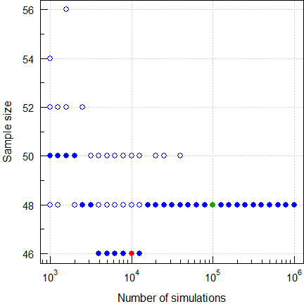

Fig. 12 Sample size for RSABE (2×2×4 replicate, CV 0.70, GMR 0.90, power ≥0.90).

Five runs. Filled circles are with a fixed seed of 123456 and open circles with random seeds. With only 10,000 simulations I didn’t get 46 (like ‘The Two Lászlós’) but once 48, twice 50, once 52, and once 54. In 1,000 runs of 10,000 I got a median of 48 and a range of 44–52. With more simulations we end up with 48 as a stable result.

top of section ↩︎ previous example ↩︎ previous section ↩︎

Caveats, Hints

A regulator once told me:

»I don’t believe in simulations.«

Strong view. I doubt that he avoids to use any kind of modern transportation – a lot of simulations involved in design and testing. However, there’s a grain of truth in his statement.

“Garbage in, garbage out.
It’s very very simple.
ElMaestro (2009)¹⁴

If an analytical solution exists or more efficient methods are available, it’s easy to check whether the result of a simulation is reliable.

General

If an analytical solution exists and the calculation is reasonably fast, use it. In such a case performing simulations is a waste of time. If an exact method does not exist, it get’s tricky, i.e., rigorous testing is of utmost importance.

In statistics understanding of the data generating process helps us to decide which test we should use.

Concentrations – and hence, an integrated pharmacokinetic metric as the AUC as well – likely follow a lognormal distribution. Hence, in order to apply methods requiring normal distributed data, we log_e-transform them first.
The variance follows a χ²-distribution.
Time points of observations (t_max, t_lag) depend on the sampling schedule and therefore, are discrete (although the distribution of the true ones is continuous; for details see this article).

Given that, in simulations we have take the distributional properties into account. It would be a serious flaw to simply fire up rnorm(n, mean = 0, sd = 1) in R, simulating the standard normal $\small{\mathcal{N}(0,1)}$.

As said above, in the simulation-functions of PowerTOST these ‘key’ statistics are implemented: $\small{\sigma^2}$ follows a $\small{\chi^2\textrm{-}}$distribution with $\small{n-2}$ degrees of freedom and $\small{\log_{e}(\theta_0)}$ follows a normal distribution. This approach is less computationally intensive than simulating subjects of a study.

Let’s compare the sample size, power, and empiric Type I Error for a 4-period full replicate design, homoscedasticity $\small{(CV_\textrm{wT}=CV_\textrm{wR}=0.45)}$, T/R-ratio 0.90, target power ≥ 0.80, intended for the EMA’s ABEL.

CV           <- 0.45
design       <- "2x2x4"
U            <- scABEL(CV = CV)[["upper"]]
comp         <- data.frame(method = c("stats", "subj"),
                           n = NA, power = NA, TIE = NA,
                           secs = NA)
st           <- proc.time()[[3]]
comp[1, 2:3] <- sampleN.scABEL(CV = CV, design = design,
                               details = FALSE,
                               print = FALSE)[8:9]
comp[1, 4]   <- power.scABEL(CV = CV, design = design,
                             n = comp$n[1], theta0 = U,
                             nsims = 1e6)
comp[1, 5]   <- proc.time()[[3]] - st
st           <- proc.time()[[3]]
comp[2, 2:3] <- sampleN.scABEL.sdsims(CV = CV,
                                      design = design,
                                      details = FALSE,
                                      print = FALSE)[8:9]
comp[2, 4]   <- power.scABEL.sdsims(CV = CV,
                                    design = design,
                                    n = comp$n[1],
                                    theta0 = U,
                                    nsims = 1e6,
                                    progress = FALSE)
comp[2, 5]   <- proc.time()[[3]] - st
comp[1]      <- c("\u2018key\u2019 stat\u2019s",
                  "subject sim\u2019s")
print(comp, row.names = FALSE)

#         method  n   power      TIE  secs
#   ‘key’ stat’s 28 0.81116 0.048889  0.77
#  subject sim’s 28 0.81196 0.048334 35.85

That’s a sufficiently close match and in general simulating via the ‘key’ statistics is justified due to speed reasons.

However, there is one scenario where subject simulations are recommended: A partial replicate design intended for ABEL assuming heteroscedasticity (if and only if $\small{CV_\textrm{wT}>CV_\textrm{wR})}$.

CV           <- 0.45
# split based on the variance ratio,
# first element CVwT, second element CVwR
CV           <- CVp2CV(CV, ratio = 1.5)
design       <- "2x3x3"
U            <- scABEL(CV = CV[2])[["upper"]]
comp         <- data.frame(method = c("stats", "subj"),
                           CVwT = CV[1], CVwR = CV[2],
                           n = NA, power = NA, TIE = NA,
                           secs = NA)
st           <- proc.time()[[3]]
comp[1, 4:5] <- sampleN.scABEL(CV = CV, design = design,
                               details = FALSE,
                               print = FALSE)[8:9]
comp[1, 6]   <- power.scABEL(CV = CV, design = design,
                             n = comp$n[1], theta0 = U,
                             nsims = 1e6)

# Warning: Heteroscedasticity in the 2x3x3 design may lead to poor accuracy of power;
# consider the function power.scABEL.sdsims() instead.

comp[1, 7]   <- proc.time()[[3]] - st
st           <- proc.time()[[3]]
comp[2, 4:5] <- sampleN.scABEL.sdsims(CV = CV,
                                      design = design,
                                      details = FALSE,
                                      print = FALSE)[8:9]
comp[2, 6]   <- power.scABEL.sdsims(CV = CV,
                                    design = design,
                                    n = comp$n[1],
                                    theta0 = U, nsims = 1e6,
                                    progress = FALSE)
comp[2, 7]   <- proc.time()[[3]] - st
comp[, 2:3]  <- signif(comp[, 2:3], 4)
comp[1]      <- c("\u2018key\u2019 stat\u2019s",
                  "subject sim\u2019s")
print(comp, row.names = FALSE)

#         method   CVwT   CVwR  n   power      TIE  secs
#   ‘key’ stat’s 0.4977 0.3987 51 0.81558 0.054635  0.60
#  subject sim’s 0.4977 0.3987 54 0.81723 0.067935 60.85

THX to the authors of the package for warning us and suggesting an alternative!
Actually we need three more subjects. Yes, the Type I Error is inflated. It is discussed in another article.

Compare that with homoscedasticity.

CV           <- c(0.45, 0.45)
design       <- "2x3x3"
U            <- scABEL(CV = CV[2])[["upper"]]
comp         <- data.frame(method = c("stats", "subj"),
                           CVwT = CV[1], CVwR = CV[2],
                           n = NA, power = NA, TIE = NA,
                           secs = NA)
st           <- proc.time()[[3]]
comp[1, 4:5] <- sampleN.scABEL(CV = CV, design = design,
                               details = FALSE,
                               print = FALSE)[8:9]
comp[1, 6]   <- power.scABEL(CV = CV, design = design,
                             n = comp$n[1], theta0 = U,
                             nsims = 1e6)
comp[1, 7]   <- proc.time()[[3]] - st
st           <- proc.time()[[3]]
comp[2, 4:5] <- sampleN.scABEL.sdsims(CV = CV,
                                      design = design,
                                      details = FALSE,
                                      print = FALSE)[8:9]
comp[2, 6]   <- power.scABEL.sdsims(CV = CV,
                                    design = design,
                                    n = comp$n[1],
                                    theta0 = U,
                                    nsims = 1e6,
                                    progress = FALSE)
comp[2, 7]   <- proc.time()[[3]] - st
comp[, 2:3]  <- signif(comp[, 2:3], 4)
comp[1]      <- c("\u2018key\u2019 stat\u2019s",
                  "subject sim\u2019s")
print(comp, row.names = FALSE)

#         method CVwT CVwR  n   power      TIE  secs
#   ‘key’ stat’s 0.45 0.45 39 0.80588 0.046774  0.65
#  subject sim’s 0.45 0.45 39 0.80256 0.048737 41.16

No problems even in a partial replicate design.

Why do we need fewer subjects? Although with heteroscedasticity we had the same pooled $\small{CV_\textrm{w}}$ of 0.45, here we can expand the limits more ($\small{CV_\textrm{wR}=0.45\rightarrow 72.15-138.59\%}$ than with $\small{CV_\textrm{wR}=0.3987\rightarrow 74.68-133.90\%}$) and the lower $\small{CV_\textrm{wT}}$ (0.45 instead of 0.4977) will result in a narrower 90% confidence interval.

top of section ↩︎ previous section ↩︎

Documentation

Welcome to the nightmare. What you should do:

PRNG: Pseudorandom number generator.

Use a fixed seed of the PRNG and give it in protocols, reports, and publications. State also the number of simulations. Only then results can be reproduced.
- From an infamous example:
  »A different randomly selected seed was used for each scenario.«
  Of course, I value the paper¹¹ – though it should have been published in the Journal of Irreproducible Results in parallel. Given, one can almost reproduce the results but only if rounded to three significant digits.
- An R-package for bootstrapping the similarity factor f₂ implemented only a random seed.¹⁵ ¹⁶ I have seen deficiency letters because regulatory assessors failed to reproduce the reported result.¹⁷ Gratefully in later versions a fixed seed is implemented¹⁸ and the package considered acceptable.¹⁹
- In one of our manuscripts²⁰ a reviewer remarked:
  »The authors report the statistical precision of their simulation results, generators, random seeds, etc. which is frequently forgotten in other simulation studies.«
  THX for the flowers!
State which PRNG you used.
- Nowadays in most software the Mersenne Twister ²¹ is the default. With its period of ≈4.3×10^6,001 one can be sure to get no repetitions in even extremely large simulations. Since v2010 it is implemented in M$ Excel.
- In VBA still a linear congruential generator is implemented, which is useless in large Monte Carlo simulations due to its short period. Hence, be cautious if you use simulations based on macros.
Find a compromise between accuracy and speed.
- Software should support both fixed and random seeds (e.g., the R-packages PowerTOST,³ Power2Stage,⁴ and randomizeBE²²). Where the former (ideally as the default) facilitates reproducibility, the latter can be used to assess the stability of results and find a suitable number of simulations.
- As shown above, 100,000 simulations are sufficient in sample size estimations for SABE. In simulating the empiric Type I Error (e.g., for SABE, adaptive Two-Stage Designs) one million simulations are highly recommended and the standard nowadays.

For geeks and neRs only:

Let us explore the tables¹² in detail.

László Tóthfalusi coded in MatLab. The seed of the PRNG is not given in the paper. Though the Mersenne Twister is the standard PRNG of MatLab (like in R), its implementations might be different. Even with the same seed and the same number of simulations different results may be obtained.
An example: Power in simulations is given by the number of passing studies divided by the number of simulations. Say, we aim at 80% power in a partial replicate design and get in one software 0.80000 and in another 0.79999. The first software will stop and estimate a sample size of n, whereas the second would continue to n + 3.
Another discrepancy arises from the fact that all sample size functions of PowerTOST return balanced sequences, whereas the authors reported the smallest sample size which gives at least the desired power. Therefore, in Tables A1/A3 you find some even numbers (for three sequences) and in Tables A2/A4 some odd numbers (for two sequences), whereas sampleN.RSABE() and sampleN.scABEL() round up to the next multiple of three and two, respectively.
The authors simulated subjects, whereas in sampleN.RSABE() / sampleN.scABEL() the ‘key’ statistics are used. The latter approach can be up to 100 times faster than the former.
- For ABEL subject simulations are provided by the function sampleN.scABEL.sdsims(). Only if you suspect heterogenicity (i.e., give CV as a vector with two elements, where the first one is CV_wT and the second CV_wR), you plan a partial replicate design, and CV_wT > CV_wR, that is the method of choice. If CV_wT ≤ CV_wR and for all full replicate designs I recommend sampleN.scABEL() for speed reasons. See also the package’s vignette.²³
- Sorry, subject simulations are not possible for the FDA’s RSABE. Since the FDA’s mixed-effects model for ABE (mandatory if s_wR < 0.294) cannot be set up in R, intra-subject contrasts are used. However, it is a reasonably close approximation. For a comparison with SAS see page 16 of the file Implementation_scaledABE_sims.pdf in the folder /library/PowerTOST/doc.
Possibly the authors used a rounded regulatory constant (0.893) instead of the exact value (log_e(1.25)/0.25 = 0.8925742…) like sampleN.RSABE() does. In recalculating the entire tables with 0.893 (100,000 simulations) we found five of the 352 scenarios where the sample size would be by one sequence smaller. However, I would not go that way because if you will evaluate the study with the SAS-code of the FDA²⁴ ²⁵ or the template for Phoenix WinNonlin, the exact regulatory constant will be used.
Another question is at which CV_wR (on the average) the simulations switch from ABE to SABE. The following code compares sample sizes for ABE and RSABE or ABE (example for a T/R-ratio 0.90, target power ≥ 0.80).

fun1 <- function(x) {
  n.1 <- sampleN.TOST(CV = x, theta0 = theta0,
                      targetpower = target,
                      design = design, details = FALSE,
                      print = FALSE)[["Sample size"]]
  n.2 <- sampleN.RSABE(CV = x, theta0 = theta0,
                       targetpower = target,
                       design = design, details = FALSE,
                       print = FALSE)[["Sample size"]]
  return(n.1 - n.2)
}
fun2 <- function(x) {
  n.1 <- sampleN.TOST(CV = x, theta0 = theta0,
                      targetpower = target,
                      design = design, details = FALSE,
                      print = FALSE)[["Sample size"]]
  n.2 <- sampleN.scABEL(CV = x, theta0 = theta0,
                        targetpower = target,
                        design = design, details = FALSE,
                        print = FALSE)[["Sample size"]]
  return(n.1 - n.2)
}
theta0 <- 0.90
target <- 0.80
design <- "2x2x4"
cat("2-sequence 4-period full replicate design",
    sprintf("\n  Equal sample sizes for ABE and RSABE at CV = %.1f%%.",
    100 * uniroot(fun1, interval = c(0.3, 0.4), extendInt = "yes")$root),
    sprintf("\n  Equal sample sizes for ABE and ABEL  at CV = %.1f%%.",
    100 * uniroot(fun2, interval = c(0.3, 0.4), extendInt = "yes")$root), "\n")
design <- "2x2x3"
cat("2-sequence 3-period full replicate design",
    sprintf("\n  Equal sample sizes for ABE and RSABE at CV = %.1f%%.",
    100 * uniroot(fun1, interval = c(0.3, 0.4), extendInt = "yes")$root),
    sprintf("\n  Equal sample sizes for ABE and ABEL  at CV = %.1f%%.",
    100 * uniroot(fun2, interval = c(0.3, 0.4), extendInt = "yes")$root), "\n")
design <- "2x3x3"
cat("3-sequence 3-period partial replicate design",
    sprintf("\n  Equal sample sizes for ABE and RSABE at CV = %.1f%%.",
    100 * uniroot(fun1, interval = c(0.3, 0.4), extendInt = "yes")$root),
    sprintf("\n  Equal sample sizes for ABE and ABEL  at CV = %.1f%%.",
    100 * uniroot(fun2, interval = c(0.3, 0.4), extendInt = "yes")$root), "\n")

# 2-sequence 4-period full replicate design 
#   Equal sample sizes for ABE and RSABE at CV = 25.5%. 
#   Equal sample sizes for ABE and ABEL  at CV = 20.7%. 
# 2-sequence 3-period full replicate design 
#   Equal sample sizes for ABE and RSABE at CV = 20.7%. 
#   Equal sample sizes for ABE and ABEL  at CV = 20.7%. 
# 3-sequence 3-period partial replicate design 
#   Equal sample sizes for ABE and RSABE at CV = 25.5%. 
#   Equal sample sizes for ABE and ABEL  at CV = 27.9%.

Given that, it hardly matters for true HVD(P)s. Note that the tables don’t reach below 30% and the authors stated in the discussion:

»In view of the consequences of the mixed approach, it could be judicious to consider larger numbers of subjects at variations fairly close to 30%.«

top of section ↩︎ previous section ↩︎

Acknowledgment

Member ElMaestro of the BEBA-Forum for calculating the exact probability of observing pre-dose concentrations > LLOQ and Detlew Labes for discovering a bug in my power of TOST-simulations.

Licenses

Helmut Schütz 2024
R and packages GPL 3.0,TeachingDemos Artistic 2.0, klippy MIT, pandoc GPL 2.0.
1^st version March 13, 2021. Rendered April 8, 2024 00:27 CEST by rmarkdown via pandoc in 0.60 seconds.

Footnotes and References

Snow G. TeachingDemos: Demonstrations for Teaching and Learning. Package version 2.13. 2024-02-13. CRAN.↩︎
Robotham A. magicaxis: Pretty Scientific Plotting with Minor-Tick and Log Minor-Tick Support. Package version 2.4.5. 2024-01-29. CRAN.↩︎
Labes D, Schütz H, Lang B. PowerTOST: Power and Sample Size for (Bio)Equivalence Studies. Package version 1.5.6. 2024-03-18. CRAN.↩︎
Labes D, Lang B, Schütz H. Power2Stage: Power and Sample-Size Distribution of 2-Stage Bioequivalence Studies. Package version 0.5.4. 2021-11-20. CRAN.↩︎
Pinheiro J, Bates D, DebRoy S, Sarkar D, EISPACK authors, Heisterkamp S, Van Willigen B, Ranke J, R-core. nlme: Linear and Nonlinear Mixed Effects Models. Package version 3.1.164. 2023-11-27. CRAN.↩︎
Bates D, Maechler M, Bolker B, Walker S, Christensen RHB, Singmann H, Dai B, Scheipl F, Grothendieck G, Green P, Fox J, Bauer A, Krivitsky PN. lme4: Linear Mixed-Effects Models using ‘Eigen’ and S4. Package version 1.1.35.2. 2024-03-28. CRAN.↩︎
Kuznetsova A, Brockhoff PB, Haubo Bojesen Christensen R, Pødenphant Jensen S. lmerTest: Tests in Linear Mixed Effects Models. Package version 3.1.3. 2020-10-23. CRAN.↩︎
Jensen R. Simulating Buffon’s Needle in R. 2019-12-18. Answer at StackExchange.↩︎
Zheng C, Wang J, Zhao L. Testing bioequivalence for multiple formulations with power and sample size calculations. Pharm Stat. 2012; 11(4): 334–41. doi:10.1002/pst.1522.↩︎
Schütz H. Two-stage designs in bioequivalence trials. Eur J Clin Pharmacol. 2015; 71(3): 271–81. doi:10.1007/s00228-015-1806-2.↩︎
Potvin D, DiLiberti CE, Hauck WW, Parr AF, Schuirmann DJ, Smith RA. Sequential design approaches for bioequivalence studies with crossover designs Pharm Stat. 2007; 7(4): 245–262. doi:10.1002/pst.294.↩︎
Tóthfalusi L, Endrényi L. Sample Sizes for Designing Bioequivalence Studies for Highly Variable Drugs. J Pharm Pharmaceut Sci. 2011; 15(1): 73–84. doi:10.18433/j3z88f. Open access.↩︎
If you perform five runs with 10,000 simulations, you will get different numbers. That’s the effect of random seeds and a low number of simulations.↩︎
ElMaestro. Why not use R? BEBA Forum. January 2009. Online.↩︎
Mendyk A. bootf2BCA. SourceForge.↩︎
Schütz H. bootf2BCA v1.1. BEBA-Forum. 2019-10-05. Online.↩︎
Same operating system, same version of the package, same data, same number of bootstraps. Only the seed of the PRNG differed…↩︎
Schütz H. bootf2BCA v1.2: seed. BEBA-Forum. 2020-09-25. Online.↩︎
Noce V, Gwaza L, Mangas-Sanjuan V, García-Arieta A. Comparison of free software platforms for the calculation of the 90% confidence interval of f₂ similarity factor by bootstrap analysis. Eur J Pharm Sci. 2020; 146: 10529. doi:10.1016/j.ejps.2020.105259.↩︎
Schütz H, Labes D, Wolfsegger MJ. Critical Remarks on Reference-Scaled Average Bioequivalence. J Pharm Pharmaceut Sci. 25: 285–96. doi:10.18433/jpps32892. Open access.↩︎
Matsumoto M, Nishimura T. Mersenne Twister: A 623-dimensionally equidistributed uniform pseudo-random number generator. ACM Trans Model Comput Simul. 1998; 8: 3–30. doi:10.1145/272991.272995.↩︎
Labes D. randomizeBE: Create a Random List for Crossover Studies. Package version 0.3.6. 2023-08-19. CRAN.↩︎
Schütz H. Reference-Scaled Average Bioequivalence. Heterogenicity. 2022-02-19. CRAN.↩︎
FDA, OGD. Draft Guidance on Progesterone. Rockville. Recommended Apr 2010; Revised Feb 2011. Download.↩︎
FDA, CDER. Draft Guidance for Industry. Bioequivalence Studies With Pharmacokinetic Endpoints for Drugs Submitted Under an ANDA. Silver Spring. August 2021. Download.↩︎

Simulations 101

Helmut Schütz

April 8, 2024

Introduction

Examples

Rolling two dice

Estimating π

LLOQ

TOST and its relatives

Power

Type I Error

Period / sequence effects

Equal carryover

Unequal carryover

Sample size for SABE

ABEL

RSABE

Caveats, Hints

General

Documentation

Acknowledgment

Licenses

Footnotes and References