
Sample Size Estimation for Equivalence Studies Intended for ABEL
Helmut Schütz

April 10, 2025
Consider allowing JavaScript. Otherwise, you have to be proficient in
reading  since formulas
will not be rendered. Furthermore, the table of contents in the left
column for navigation will not be available and code-folding not
supported. Sorry for the inconvenience.
since formulas
will not be rendered. Furthermore, the table of contents in the left
column for navigation will not be available and code-folding not
supported. Sorry for the inconvenience.
Examples in this article were generated with
 4.4.3
by the package
4.4.3
by the package PowerTOST.1
More examples are given in the respective vignette.2 See also the README on GitHub for an overview and the online manual3 for details.
The right-hand badges give the respective section’s ‘level’.
- Basics about sample size methodology – requiring no or only limited statistical expertise.
- These sections are the most important ones. They are – hopefully – easily comprehensible even for novices.
- A somewhat higher knowledge of statistics and/or R is required. May be skipped or reserved for a later reading.
- An advanced knowledge of statistics and/or R is required. Not recommended for beginners in particular.
- If you are not a neRd or statistics afficionado, skipping is recommended. Suggested for experts but might be confusing for others.
- Click to show / hide R code.
- Click on the icon
 in the top left corner to copy R code to the
clipboard.
in the top left corner to copy R code to the
clipboard.
Abbreviations are given at the end.
Introduction
What is Average Bioequivalence with Expanding Limits?
For details about inferential statistics and hypotheses in equivalence see another article.
Definitions:
- A Highy Variable Drug (HVD) shows a within-subject Coefficient of Variation \(\small{(CV_\text{wR})}\) \(\small{>30\%}\) if administered as a solution in a replicate design. The high variability is an intrinsic property of the drug (absorption/permeation, clearance).
- A Highy Variable Drug Product (HVDP) shows a \(\small{CV_\text{wR}>30\%}\) in a replicate design.4
The concept of Scaled Average Bioequivalence (SABE) for HVDPs is based on the following considerations:
- HVDPs are safe
and efficacious despite their high variability because:
- They have a wide therapeutic index (i.e., a flat
dose-response curve). Consequently, even substantial changes in
concentrations have only a limited impact on the effect.
If they would have a narrow therapeutic index, adverse effects (due to high concentrations) and lacking effects (due to low concentrations) would have been observed in Phase III and consequently, the originator’s product should not have been approved in the first place.5 - Once approved, the product has a documented safety / efficacy record
in phase IV and in clinical practice – despite its high
variability.
If problems were evident, the product would have been taken off the market.
- They have a wide therapeutic index (i.e., a flat
dose-response curve). Consequently, even substantial changes in
concentrations have only a limited impact on the effect.
- Given that, the conventional ‘clinically relevant difference’ \(\small{\Delta}\) of 20% (leading to the limits of 80.00 – 125.00% in Average Bioequivalence) is overly conservative and thus, leading to large sample sizes.
- Hence, a more relaxed \(\small{\Delta>20\%}\) was proposed. A natural approach is to scale (expand / widen) the limits based on the within-subject variability of the reference product \(\small{s_\text{wR}}\). In this approach, power for a given sample size would be ideally independent from the variability.
The conventional confidence interval inclusion approach in ABE \[\begin{matrix}\tag{1} \theta_1=1-\Delta,\theta_2=\left(1-\Delta\right)^{-1}\\ H_0:\;\frac{\mu_\text{T}}{\mu_\text{R}}\ni\left\{\theta_1,\theta_2\right\}\;vs\;H_1:\;\theta_1<\frac{\mu_\text{T}}{\mu_\text{R}}<\theta_2\textsf{,}, \end{matrix}\] where \(\small{H_0}\) is the null hypothesis of inequivalence and \(\small{H_1}\) the alternative hypothesis, \(\small{\theta_1}\) and \(\small{\theta_2}\) are the fixed lower and upper limits of the acceptance range, and \(\small{\mu_\text{T}}\) are the geometric least squares means of \(\small{\text{T}}\) and \(\small{\text{R}}\), respectively is in Scaled Average Bioequivalence (SABE)6 modified to \[H_0:\;\frac{\mu_\text{T}}{\mu_\text{R}}\Big{/}\sigma_\text{wR}\ni\left\{\theta_{\text{s}_1},\theta_{\text{s}_2}\right\}\;vs\;H_1:\;\theta_{\text{s}_1}<\frac{\mu_\text{T}}{\mu_\text{R}}\Big{/}\sigma_\text{wR}<\theta_{\text{s}_2}\textsf{,}\tag{2}\] where \(\small{\sigma_\text{wR}}\) is the standard deviation of the reference and the scaled limits \(\small{\left\{\theta_{\text{s}_1},\theta_{\text{s}_2}\right\}}\) of the acceptance range depend on conditions given by the agency.
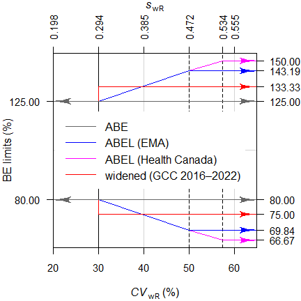
Average Bioequivalence with Expanding Limits (ABEL)7 for HVDPs is acceptable in numerous jurisdictions (Fig. 2), whereas directly widening the limits was recommended 2016 – 2022 in the member states of the Gulf Cooperation Council8 (Fig. 3). Alas, we are far away from global harmonization. Work on the ICH’s M13C guideline9 started in February 2025. Consensus on the Technical Document (Step 2a/2b) is proposed for June 2027 and adoption of the harmonised guideline (Step 4) for February 2029.10
Expanding the limits is acceptable for different pharmacokinetic metrics.
| PK metric | Jurisdiction |
|---|---|
| Cmax | The EEA,11 the WHO,12 13 Australia,14 Belarus,15 the EAC,16 the ASEAN states,17 the Russian Federation,18 the EEU,19 Egypt,20 New Zealand,21 Chile,22 Brazil,23 members of the GCC,24 Mexico.25 |
| AUC | WHO (if in a 4-period full replicate design),12 Canada.26 | Cmin, Cτ | The EEA (controlled release products in steady state).27 | partial AUC | The EEA (controlled release products).27 |
Based on the switching \(\small{CV_0=30\%}\) we get the switching standard deviation \(\small{s_0=\sqrt{\log_{e}(CV_{0}^{2}+1)}\approx0.2935604\ldots}\), the (rounded) regulatory constant \(\small{k=\frac{\log_{e}1.25}{s_0}\sim0.76}\), and finally the expanded limits \(\small{\left\{\theta_{\text{s}_1},\theta_{\text{s}_2}\right\}=}\) \(\small{100\left(\exp(\mp0.76\cdot s_{\text{wR}})\right)}\). Note that in the guidelines the terminology \(\small{\left\{\text{L},\text{U}\right\}}\) is used instead.
In order to apply the methods following conditions have to be fulfilled:
- The study has to be performed in a replicate design (i.e., at least the reference product has to be administered twice).
- A clinical justification has to be provided that the expanded limits will not impact safety / efficacy.
- The observed within-subject variability of the reference \(\small{(CV_\text{wR})}\) has to be > 30%.
- Except in Chile and Brazil, it has to be demonstrated that the high variability is not caused by ‘outliers’. This topic will be covered in another article.
The wording in the guidelines gives the false impression that the methods are straightforward. In fact they are decision schemes (frameworks), which hinge on the estimated standard deviation of the reference treatment \(\small{s_{\text{wR}}}\).
If \(\small{CV_\text{wR}\leq30\%}\) the study has to be assessed for ABE (left branch) or for ABEL (right branch) otherwise.
In the ABEL-branch there is an ‘upper cap’ of scaling (\(\small{uc=50\%}\) in all jurisdictions except for Health Canada, where \(\small{uc\approx 57.382\%}\)). Furthermore, the point estimate (\(\small{PE}\)) has to lie within 80.00 – 125.00%.

Fig. 2 Decision scheme of the EMA, Health Canada, …
From March 2016 to August 2022 the GCC recommended a simplified variant with fixed widened limits of 75.00 – 133.33% if \(\small{CV_\text{wR}>30\%}\).8 Like in ABEL the \(\small{PE}\) had to lie within 80.00 – 125.00%. As in the FDA’s RSABE there was no ‘upper cap’.
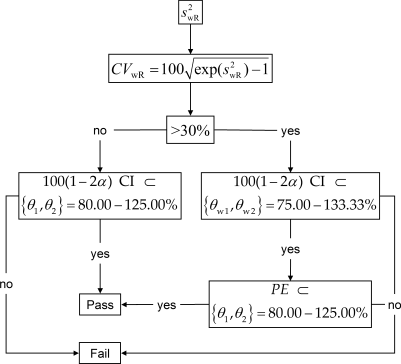
Fig. 3 Former decision scheme of the GCC.
Since the applicability of these approaches hinges on the realized values (\(\small{CV_\text{wR}}\), \(\small{PE}\)) in the particular study – which are random variables and as such unknown beforehand – analytical solutions for power (and hence, the sample size) do not exist. Therefore, extensive simulations of potential combinations have to be employed.
Whereas ABE is bijective (if \(\small{T}\) is equivalent to \(\small{R}\), \(\small{R}\) is also equivalent to \(\small{T}\)), this holds in ABEL only if \(\small{CV_\text{wT}=}\) \(\small{CV_\text{wR}}\). Therefore, switching from \(\small{R}\) to \(\small{T}\) is tolerable if \(\small{CV_\text{wT}<CV_\text{wR}}\) but switching from \(\small{T}\) to \(\small{R}\) can be problematic. Individual Bioequivalence (IBE) would not only compare the averages of products but also their variances and thus, support ‘Switchability’.28 However, IBE was never implemented in regulatory practice. For details see this article.
Cave: Under certain conditions the methods may lead to an inflated Type I Error, i.e., an increased patient’s risk29 30 (for details see another article). Two approaches of dealing with this problem are presented below.
For the evaluation I recommend the package
replicateBE.31
Interlude 1
Where do these numbers come from?
With the regulatory constant \(\small{k=0.76}\) one gets in the \(\small{\log_{e}}\)-scale a linear expansion
from \(\small{CV_\text{wR}=30\%}\) to
\(\small{uc}\) based on \(\small{s_\text{wR}=\sqrt{\log_{e}(CV_\text{wR}^{2})+1}}\)
and \(\small{100\left(\exp(\mp k\cdot
s_\text{wR})\right)}\).
Hence, with \(\small{CV_\text{wR}=30\%}\) one gets
\(\small{\;\;\;\left\{\theta_1,\theta_2\right\}=100\left(\exp(\mp0.76\cdot
0.2935604)\right)=\left\{80.00,\,125.00\right\}}\).
With \(\small{uc=50\%}\) one gets
\(\small{\;\;\;\left\{\theta_{\text{s}_1},\,\theta_{\text{s}_2}\right\}=100\left(\exp(\mp0.76\cdot
0.4723807)\right)=\left\{69.83678,\,143.19102\right\}}\).
For Health Canada with \(\small{uc=57.382\%}\) one gets \(\small{\;\;\;\left\{\theta_{\text{s}_1},\,\theta_{\text{s}_2}\right\}=100\left(\exp(\mp0.76\cdot
0.5335068)\right)=\left\{66.66667,\,150.00000\right\}}\).
As stated above, the regulatory constant \(\small{k}\) is given in all guidelines rounded to two significant digits. Based on the switching \(\small{CV_\text{w0}=30\%}\) one gets \(\small{s_\text{w0}=\sqrt{\log_{e}(CV_\text{w0}^2+1)}\approx 0.2935604}\) and, therefore, the exact value would be \(\small{k=\frac{\log_{e}1.25}{s_\text{w0}}\approx 0.7601283}\). For a rant see Karalis et al.32 The wisdom of regulators is unfathomable.
A clinically not relevant \(\small{\Delta}\) of 30% (leading a fixed
range of 70.00 – 142.86%) was acceptable in Europe (in exceptional cases
even for AUC) if pre-specified in the protocol. A replicate
design was not required.33 34 35
A clinically not relevant \(\small{\Delta}\) of 25% for
Cmax (75.00 – 133.33%) was acceptable for the
EMA if the study was
performed in a replicate design and \(\small{CV_\text{wR}>30\%}\).36 A \(\small{\Delta}\) of 25% for
Cmax (75.00 – 133.33%) is currently acceptable in
South Africa,37 by the League of Arab States,38 and was
acceptable in Kazakhstan.39
Hence, this excursion into history may explain the upper cap of scaling
in
ABEL
and the (former) widened limits for the
GCC. I assume that Health
Canada’s 66.7 – 150.0% are no more than ‘nice
numbers’ – as usual.40
Preliminaries
A basic knowledge of R is
required. To run the scripts at least version 1.4.8 (2019-08-29) of
PowerTOST is required and at least version 1.5.3
(2021-01-18) suggested. Any version of R would
likely do, though the current release of PowerTOST was only
tested with R 4.3.3 (2024-02-29) and later.
All scripts were run on a Xeon E3-1245v3 @ 3.40GHz (1/4 cores) 16GB RAM
with R 4.4.3 on Windows 7 build 7601, Service
Pack 1.
Note that in all functions of PowerTOST the arguments
(say, the assumed T/R-ratio theta0, the assumed coefficient
of variation CV, etc.) have to be given as ratios and not
in percent.
sampleN.scABEL() gives balanced sequences
(i.e., an equal number of subjects is allocated to all
sequences). Furthermore, the estimated sample size is the total
number of subjects – and not the number of subjects per sequence like in
some other software packages.
All examples deal with studies where the response variables likely follow a log-normal distribution, i.e., we assume a multiplicative model (ratios instead of differences). We work with \(\small{\log_{e}}\)-transformed data in order to allow analysis by the t-test (requiring differences).
Terminology
It may sound picky but ‘sample size calculation’ (as used in most guidelines and alas, in some publications and textbooks) is sloppy terminology. In order to get prospective power (and hence, a sample size), we need five values:
- The level of the test \(\small{\alpha}\) (in BE commonly 0.05),
- the (potentially expanded) BE-margin,
- the desired (or target) power \(\small{\pi}\),
- the variance (commonly expressed as a coefficient of variation), and
- the deviation of the test from the reference treatment,
where
- is fixed by the agency,
- depends on the observed41 \(\small{CV_\text{wR}}\) (which is unknown beforehand),
- is set by the sponsor (commonly to 0.80 – 0.90),
- is an uncertain assumption,
- is an uncertain assumption.
In other words, obtaining a sample size is not an exact calculation like \(\small{2\times2=4}\) but always just an estimation.
“Power Calculation – A guess masquerading as mathematics.
Of note, it is extremely unlikely that all assumptions will be exactly realized in a particular study. Hence, calculating retrospective (a.k.a. estimated, post hoc, a posteriori) power is not only futile but plain nonsense.43 For details see another article.
It is a prerequisite that no carryover from one period to the next exists. Only then the comparison of treatments will be unbiased.44 Carryover is elaborated in another article.
Except for Health Canada (where a mixed-effects model is required) the recommended evaluation by an ANOVA assumes homoscedasticity (\(\small{s_\text{wT}^2=s_\text{wR}^2}\)), which is – more often than not – wrong.
Power → Sample size
The sample size cannot be directly estimated, in
ABEL
only
power simulated for an already given sample size.
In contrast to ABE, where power can be exactly calculated and the sample size is determined in an iterative procedure, ABEL is a decision scheme and therefore, simulations must to performed for different combinations of assumed T/R-ratios and CVs.
“Power. That which statisticians are always calculating but never have.
Let’s start with PowerTOST.
The sample size functions’ defaults are:
| Argument | Default | Meaning |
|---|---|---|
alpha
|
0.05
|
Nominal level of the test |
targetpower
|
0.80
|
Target (desired) power |
theta0
|
0.90
|
Assumed T/R-ratio |
theta1
|
0.80
|
Lower BE-limit in ABE and lower PE-constraint in ABEL |
theta2
|
1.25
|
Upper BE-limit in ABE and upper PE-constraint in ABEL |
design
|
"2x3x3"
|
Treatments × Sequences × Periods |
regulator
|
"EMA"
|
Guess… |
nsims
|
1e05
|
Number of simulations |
print
|
TRUE
|
Output to the console |
details
|
TRUE
|
Show regulatory settings and sample size search |
setseed
|
TRUE
|
Set a fixed seed (recommended for reproducibility) |
Implemented designs are "2x3x3" (the three sequence,
three period – partial – replicate design TRR|RTR|RRT),
"2x2x4" (two sequence, four period full replicate
designs TRTR|RTRT, TRRT|RTTR, and TTRR|RRTT), and "2x2x3"
(two sequence, three period full replicate designs TRT|RTR and
TRR|RTT).
For a quick overview of the regulatory limits use the function
scABEL() – for once in percent according to the guidelines.
Note that Health Canada uses rounding to the first decimal place.
df1 <- data.frame(regulator = "EMA", CV = c(30, 50),
                  L = NA, U = NA,
                  cap = c("lower", "upper"))
df2 <- data.frame(regulator = "HC",
                  CV = c(30, 57.382),
                  L = NA, U = NA,
                  cap = c("lower", "upper"))
for (i in 1:2) {
  df1[i, 3:4] <- sprintf("%.2f%%", 100*scABEL(df1$CV[i]/100))
  df2[i, 3:4] <- sprintf("%.1f %%", 100*scABEL(df2$CV[i]/100,
                         regulator = "HC"))
}
df1$CV <- sprintf("%.3f%%", df1$CV)
df2$CV <- sprintf("%.3f%%", df2$CV)
if (packageVersion("PowerTOST") >= "1.5.3") {
  df3 <- data.frame(regulator = "GCC <2022",
                    CV = c(30, 50), L = NA, U = NA,
                    cap = c("lower", "none"))
  for (i in 1:2) {
    df3[i, 3:4] <- sprintf("%.2f%%", 100*scABEL(df3$CV[i]/100,
                           regulator = "GCC"))
  }
  df3$CV <- sprintf("%.3f%%", df3$CV)
}
if (packageVersion("PowerTOST") >= "1.5-3") {
  print(df1, row.names = F); print(df2, row.names = F); print(df3, row.names = F)
} else {
  print(df1, row.names = F); print(df2, row.names = F)
}
# regulator CV L U cap
# EMA 30.000% 80.00% 125.00% lower
# EMA 50.000% 69.84% 143.19% upper
# regulator CV L U cap
# HC 30.000% 80.0 % 125.0 % lower
# HC 57.382% 66.7 % 150.0 % upper
# regulator CV L U cap
# GCC <2022 30.000% 80.00% 125.00% lower
# GCC <2022 50.000% 75.00% 133.33% noneThe sample size functions of PowerTOST use a
modification of Zhang’s method47 for the first guess.
# Note that theta0 = 0.90 is the default
sampleN.scABEL(CV = 0.45, targetpower = 0.80,
               design = "2x2x4", details = TRUE)
#
# +++++++++++ scaled (widened) ABEL +++++++++++
# Sample size estimation
# (simulation based on ANOVA evaluation)
# ---------------------------------------------
# Study design: 2x2x4 (4 period full replicate)
# log-transformed data (multiplicative model)
# 1e+05 studies for each step simulated.
#
# alpha = 0.05, target power = 0.8
# CVw(T) = 0.45; CVw(R) = 0.45
# True ratio = 0.9
# ABE limits / PE constraint = 0.8 ... 1.25
# EMA regulatory settings
# - CVswitch = 0.3
# - cap on scABEL if CVw(R) > 0.5
# - regulatory constant = 0.76
# - pe constraint applied
#
#
# Sample size search
# n power
# 24 0.7539
# 26 0.7846
# 28 0.8112An alternative to simulating the ‘key statistics’ is by subject data
simulations via the function sampleN.scABEL.sdsims().
However, it comes with a price, speed.
#               method  n   power rel.speed
#     ‘key statistics’ 28 0.81116       1.0
# subject simulations 28 0.81196 21.5Examples
Throughout the examples I’m referring to studies in a single center – not multiple groups within them or multicenter studies. That’s another pot of tea.
A Simple Case
We assume a CV of 0.45, a T/R-ratio of 0.90, a target a power of 0.80, and want to perform the study in a two sequence four period full replicate study (TRTR|RTRT or TRRT|RTTR or TTRR|RRTT) for the EMA’s ABEL.
Since theta0 = 0.90,48 targetpower = 0.80, and
regulator = "EMA" are defaults of the function, we don’t
have to give them explicitely. As usual in bioequivalence,
alpha = 0.05 is employed (we will assess the study by a
\(\small{100\,(1-2\,\alpha)=90\%}\)
confidence interval). Hence, you need to specify only the
CV (assuming \(\small{CV_\text{wT}=CV_\text{wR}}\)) and
design = "2x2x4".
To shorten the output, use the argument
details = FALSE.
#
# +++++++++++ scaled (widened) ABEL +++++++++++
#             Sample size estimation
#    (simulation based on ANOVA evaluation)
# ---------------------------------------------
# Study design: 2x2x4 (4 period full replicate)
# log-transformed data (multiplicative model)
# 1e+05 studies for each step simulated.
#
# alpha  = 0.05, target power = 0.8
# CVw(T) = 0.45; CVw(R) = 0.45
# True ratio = 0.9
# ABE limits / PE constraint = 0.8 ... 1.25
# Regulatory settings: EMA
#
# Sample size
#  n     power
# 28   0.8112
Sometimes we are not interested in the entire output and want to use
only a part of the results in subsequent calculations. We can suppress
the output by stating the additional argument print = FALSE
and assign the result to a data frame (here x).
Let’s retrieve the column names of x:
names(x)
#  [1] "Design"         "alpha"          "CVwT"
#  [4] "CVwR"           "theta0"         "theta1"
#  [7] "theta2"         "Sample size"    "Achieved power"
# [10] "Target power"   "nlast"
Now we can access the elements of x by their names. Note
that double square brackets and double or single quotes
([["…"]], [['…']]) have to be used.
Although you could access the elements by the number of the
column(s), I don’t recommend that, since in various other functions of
PowerTOST these numbers are different and hence, difficult
to remember. If you insist in accessing elements by column-numbers, use
single square brackets […].
With 28 subjects (14 per sequence) we achieve the power we desire.
What happens if we have one dropout?
# Unbalanced design. n(i)=14/13 assumed.# [1] 0.79848Below the 0.80 we desire.
Since dropouts are common, it makes sense to include / dose more subjects in order to end up with a number of eligible subjects which is not lower than our initial estimate.
Let us explore that in the next section.
Dropouts
We define two supportive functions:
- Provide equally sized sequences, i.e., any total sample
size
nwill be rounded up to achieve balance.
balance <- function(n, n.seq) {
  return(as.integer(n.seq * (n %/% n.seq + as.logical(n %% n.seq))))
}- Provide the adjusted sample size based on the original sample size
nand the anticipated droput-ratedo.rate.
In order to come up with a suggestion we have to anticipate a (realistic!) dropout rate. Note that this not the job of the statistician; ask the Principal Investigator.
“It is a capital mistake to theorise before one has data. Insensibly one begins to twist facts to suit theories, instead of theories to suit facts.
Dropout-rate
The dropout-rate is calculated from the eligible and
dosed subjects
or simply \[\begin{equation}\tag{3}
do.rate=1-n_\text{eligible}/n_\text{dosed}
\end{equation}\] Of course, we know it only after the
study was performed.
By substituting \(n_\text{eligible}\) with the estimated sample size \(n\), providing an anticipated dropout-rate and rearrangement to find the adjusted number of dosed subjects \(n_\text{adj}\) we should use \[\begin{equation}\tag{4} n_\text{adj}=\;\upharpoonleft n\,/\,(1-do.rate) \end{equation}\] where \(\upharpoonleft\) denotes rounding up to the complete sequence as implemented in the functions above.
An all too common mistake is to increase the estimated sample size \(n\) by the dropout-rate according to \[\begin{equation}\tag{5} n_\text{adj}=\;\upharpoonleft n\times(1+do.rate) \end{equation}\] If you used \(\small{(5)}\) in the past – you are not alone. In a small survey a whopping 29% of respondents reported to use it.50 Consider changing your routine.
“There are no routine statistical questions, only questionable statistical routines.
Adjusted Sample Size
In the following I specified more arguments to make the function more
flexible.
Note that I wrapped the function power.scABEL() in
suppressMessages(). Otherwise, the function will throw for
any odd sample size a message telling us that the design is
unbalanced. Well, we know that.
CV      <- 0.45 # within-subject CV
target  <- 0.80 # target (desired) power
theta0  <- 0.90 # assumed T/R-ratio
design  <- "2x2x4"
do.rate <- 0.15 # anticipated dropout-rate 15%
                # might be realively high due
                # to the 4 periods
n.seq   <- as.integer(substr(design, 3, 3))
lims    <- scABEL(CV) # expanded limits
df      <- sampleN.scABEL(CV = CV, theta0 = theta0,
                          targetpower = target,
                          design = design,
                          details = FALSE,
                          print = FALSE)
# calculate the adjusted sample size
n.adj   <- nadj(df[["Sample size"]], do.rate, n.seq)
# (decreasing) vector of eligible subjects
n.elig  <- n.adj:df[["Sample size"]]
info    <- paste0("Assumed CV              : ",
                  CV,
                  "\nAssumed T/R ratio       : ",
                  theta0,
                  "\nExpanded limits         : ",
                  sprintf("%.4f\u2026%.4f",
                  lims[1], lims[2]),
                  "\nPE constraints          : ",
                  sprintf("%.4f\u2026%.4f",
                  0.80, 1.25), # fixed in ABEL
                  "\nTarget (desired) power  : ",
                  target,
                  "\nAnticipated dropout-rate: ",
                  do.rate,
                  "\nEstimated sample size   : ",
                  df[["Sample size"]], " (",
                  df[["Sample size"]]/n.seq, "/sequence)",
                  "\nAchieved power          : ",
                  signif(df[["Achieved power"]], 4),
                  "\nAdjusted sample size    : ",
                  n.adj, " (",  n.adj/n.seq, "/sequence)",
                  "\n\n")
# explore the potential outcome for
# an increasing number of dropouts
do.act <- signif((n.adj - n.elig) / n.adj, 4)
df     <- data.frame(dosed    = n.adj,
                     eligible = n.elig,
                     dropouts = n.adj - n.elig,
                     do.act   = do.act,
                     power    = NA)
for (i in 1:nrow(df)) {
  df$power[i] <- suppressMessages(
                   power.scABEL(CV = CV,
                                theta0 = theta0,
                                design = design,
                                n = df$eligible[i]))
}
cat(info)
print(round(df, 4), row.names = FALSE)
# Assumed CV : 0.45
# Assumed T/R ratio : 0.9
# Expanded limits : 0.7215…1.3859
# PE constraints : 0.8000…1.2500
# Target (desired) power : 0.8
# Anticipated dropout-rate: 0.15
# Estimated sample size : 28 (14/sequence)
# Achieved power : 0.8112
# Adjusted sample size : 34 (17/sequence)
#
# dosed eligible dropouts do.act power
# 34 34 0 0.0000 0.8720
# 34 33 1 0.0294 0.8630
# 34 32 2 0.0588 0.8553
# 34 31 3 0.0882 0.8456
# 34 30 4 0.1176 0.8340
# 34 29 5 0.1471 0.8237
# 34 28 6 0.1765 0.8112In the worst case (six dropouts) we end up with the originally estimated sample size of 28. Power preserved, mission accomplished. If we have less dropouts, splendid – we gain power.
If we would have adjusted the sample size according to \(\small{(5)}\) we
would have dosed also 34 subjects.
Cave: This might not always be the case… If the anticipated dropout rate
of 15% is realized in the study, we would have also 28 eligible subjects
(power 0.8112). In this example we achieve still more than our target
power but the loss might be relevant in other cases.
Post hoc Power
As said in the preliminaries, calculating post hoc power is futile.
“There is simple intuition behind results like these: If my car made it to the top of the hill, then it is powerful enough to climb that hill; if it didn’t, then it obviously isn’t powerful enough. Retrospective power is an obvious answer to a rather uninteresting question. A more meaningful question is to ask whether the car is powerful enough to climb a particular hill never climbed before; or whether a different car can climb that new hill. Such questions are prospective, not retrospective.
However, sometimes we are interested in it for planning the next study.
If you give and odd total sample size n,
power.scABEL() will try to keep sequences as balanced as
possible and show in a message how that was done.
# Unbalanced design. n(i)=14/13 assumed.# [1] 0.79848Say, our study was more unbalanced. Let us assume that we dosed 34
subjects, the total number of subjects was also 27 but all dropouts
occured in one sequence (unlikely but possible).
Instead of the total sample size n we can give the number
of subjects of each sequence as a vector (the order is generally52 not
relevant, i.e., it does not matter which element refers to
which sequence).
By setting details = TRUE we can retrieve the components
of the simulations (probability to pass each test).
design   <- "2x2x4"
CV       <- 0.45
n.adj    <- 34
n.act    <- 27
n.s1     <- n.adj / 2
n.s2     <- n.act - n.s1
theta0   <- 0.90
post.hoc <- suppressMessages(
              power.scABEL(CV  = CV,
                           n = c(n.s1, n.s2),
                           theta0 = theta0,
                           design = design,
                           details = TRUE))
ABE.xact <- power.TOST(CV = CV,
                       n = c(n.s1, n.s2),
                       theta0 = theta0,
                       design = design)
sig.dig  <- nchar(as.character(n.adj))
fmt      <- paste0("%", sig.dig, ".0f (%",
                   sig.dig, ".0f dropouts)")
cat(paste0("Dosed subjects: ", sprintf("%2.0f", n.adj),
           "\nEligible      : ",
           sprintf(fmt, n.act, n.adj - n.act),
           "\n  Sequence 1  : ",
           sprintf(fmt, n.s1, n.adj / 2 - n.s1),
           "\n  Sequence 1  : ",
           sprintf(fmt, n.s2, n.adj / 2 - n.s2),
           "\nPower overall :  ",
           sprintf("%.5f", post.hoc[1]),
           "\n  p(ABEL)     :  ",
           sprintf("%.5f", post.hoc[2]),
           "\n  p(PE)       :  ",
           sprintf("%.5f", post.hoc[3]),
           "\n  p(ABE)      :  ",
           sprintf("%.5f", post.hoc[4]),
           "\n  p(ABE) exact:  ",
           sprintf("%.5f", ABE.xact), "\n"))
# Dosed subjects: 34
# Eligible : 27 ( 7 dropouts)
# Sequence 1 : 17 ( 0 dropouts)
# Sequence 1 : 10 ( 7 dropouts)
# Power overall : 0.77670
# p(ABEL) : 0.77671
# p(PE) : 0.91595
# p(ABE) : 0.37628
# p(ABE) exact: 0.37418The components of overall power are:
p(ABEL)is the probability that the confidence interval is within the expanded / widened limits.p(PE)is the probability that the point estimate is within 80.00–125.00%.p(ABE)is the probability of passing conventional Average Bioequivalence.
The line below gives the exact result obtained bypower.TOST()– confirming the simulation’s result.
Of course, in a particular study you will provide the numbers in the
n vector directly.
Lost in Assumptions
The CV and the T/R-ratio are only assumptions.
Whatever their origin might be (literature, previous studies), they
carry some degree of uncertainty. Hence, believing53 that they are the
true ones may be risky.
Some statisticians call that the ‘Carved-in-Stone’ approach.
Say, we performed a pilot study in 16 subjects and estimated the CV as 0.45.
The \(\small{\alpha}\) confidence interval of the CV is obtained via the \(\small{\chi^2}\)-distribution of its error variance \(\small{\sigma^2}\) with \(\small{n-2}\) degrees of freedom. \[\eqalign{\tag{6} s_\text{w}^2&=\log_{e}(CV_\text{w}^2+1)\\ L=\frac{(n-1)\,s_\text{w}^2}{\chi_{\alpha/2,\,n-2}^{2}}&\leq\sigma_\text{w}^2\leq\frac{(n-1)\,s_\text{w}^2}{\chi_{1-\alpha/2,\,n-2}^{2}}=U\\ \left\{lower\;CL,\;upper\;CL\right\}&=\left\{\sqrt{\exp(L)-1},\sqrt{\exp(U)-1}\right\} }\]
Let’s calculate the 95% confidence interval of the CV to get an idea.
m  <- 16 # pilot study
ci <- CVCL(CV = 0.45, df = m - 2,
           side = "2-sided", alpha = 0.05)
ci <- c(ci, mean(ci))
names(ci)[3] <- "midpoint"
signif(ci, 4)
# lower CL upper CL midpoint
# 0.3223 0.7629 0.5426Surprised? Although 0.45 is the best estimate for planning the next study, there is no guarantee that we will get exactly the same outcome. Since the \(\small{\chi^2}\)-distribution is skewed to the right, it is more likely that we will face a higher CV than a lower one in the planned study.
If we plan the study based on 0.45, we would opt for 28 subjects like
in the examples before (not adjusted for the dropout-rate).
If the CV will be lower, we loose power (less expansion). But
what if it will be higher? Depends. Since we may expand more, we gain
power. However, if we cross the upper cap of scaling (50% for the EMA),
we will loose power. But how much?
Let’s explore what might happen at the confidence limits of the CV.
m    <- 16
ci   <- CVCL(CV = 0.45, df = m - 2,
             side = "2-sided", alpha = 0.05)
n    <- 28
comp <- data.frame(CV = c(ci[["lower CL"]],
                          0.45, mean(ci),
                          ci[["upper CL"]]),
                   power = NA)
for (i in 1:nrow(comp)) {
  comp$power[i] <- power.scABEL(CV = comp$CV[i],
                                design = "2x2x4",
                                n = n)
}
comp[, 1] <- signif(comp[, 1], 4)
comp[, 2] <- signif(comp[, 2], 6)
print(comp, row.names = FALSE)
# CV power
# 0.3223 0.73551
# 0.4500 0.81116
# 0.5426 0.79868
# 0.7629 0.60158Might hurt.
What can we do? The larger the previous study was, the larger the degrees of freedom and hence, the narrower the confidence interval of the CV. In simple terms: The estimate is more certain. On the other hand, it also means that very small pilot studies are practically useless. What happens when we plan the study based on the confidence interval of the CV?
m               <- seq(12, 30, 6)
df              <- data.frame(n.pilot = m, CV = 0.45,
                              l = NA, u = NA,
                              n.low = NA, n.CV = NA, n.hi = NA)
for (i in 1:nrow(df)) {
  df[i, 3:4] <- CVCL(CV = 0.45, df = m[i] - 2,
                     side = "2-sided",
                     alpha = 0.05)
  df[i, 5] <- sampleN.scABEL(CV = df$l[i], design = "2x2x4",
                             details = FALSE,
                             print = FALSE)[["Sample size"]]
  df[i, 6] <- sampleN.scABEL(CV = 0.45, design = "2x2x4",
                             details = FALSE,
                             print = FALSE)[["Sample size"]]
  df[i, 7] <- sampleN.scABEL(CV = df$u[i], design = "2x2x4",
                             details = FALSE,
                             print = FALSE)[["Sample size"]]
}

df[, 3:4]      <- signif(df[, 3:4], 4)
names(df)[3:4] <- c("lower CL", "upper CL")
print(df, row.names = FALSE)
# n.pilot CV lower CL upper CL n.low n.CV n.hi
# 12 0.45 0.3069 0.8744 36 28 56
# 18 0.45 0.3282 0.7300 34 28 42
# 24 0.45 0.3415 0.6685 34 28 38
# 30 0.45 0.3509 0.6334 34 28 34One leading generic company has an internal rule to perform pilot studies of HVDPs in a four period full replicate design and at least 24 subjects. Makes sense.
Furthermore, we don’t know where the true T/R-ratio lies but we can calculate the lower 95% confidence limit of the pilot study’s point estimate to get an idea about a worst case. Say, it was 0.90.
m      <- 16
CV     <- 0.45
pe     <- 0.90
ci     <- round(CI.BE(CV = CV, pe = 0.90, n = m,
                      design = "2x2x4"), 4)
if (pe <= 1) {
  cl <- ci[["lower"]]
} else {
  cl <- ci[["upper"]]
}
print(cl)
# [1] 0.7515Explore the impact of a relatively 5% lower CV (less expansion) and a relatively 5% lower T/R-ratio on power for the given sample size.
n      <- 28
CV     <- 0.45
theta0 <- 0.90
comp1  <- data.frame(CV = c(CV, CV*0.95),
                     power = NA)
comp2  <- data.frame(theta0 = c(theta0, theta0*0.95),
                     power = NA)
for (i in 1:2) {
  comp1$power[i] <- power.scABEL(CV = comp1$CV[i],
                                 theta0 = theta0,
                                 design = "2x2x4",
                                 n = n)
}
comp1$power <- signif(comp1$power, 5)
for (i in 1:2) {
  comp2$power[i] <- power.scABEL(CV = CV,
                                 theta0 = comp2$theta0[i],
                                 design = "2x2x4",
                                 n = n)
}
comp2$power <- signif(comp2$power, 5)
print(comp1, row.names = FALSE)
print(comp2, row.names = FALSE)
# CV power
# 0.4500 0.81116
# 0.4275 0.80095
# theta0 power
# 0.900 0.81116
# 0.855 0.61952Interlude 2
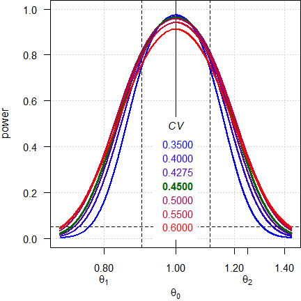
Note the log-scale of the x-axis. It demonstrates that power curves are symmetrical around 1 (\(\small{\log_{e}(1)=0}\), where \(\small{\log_{e}(\theta_2)=\left|\log_{e}(\theta_1)\right|}\)) and we will achieve the same power for \(\small{\theta_0}\) and \(\small{1/\theta_0}\) (e.g., for 0.90 and 1.1111). Contrary to ABE, power is maintained, unless we cross the upper scaling limit, where additionally the PE-constraint becomes increasingly important.
<nitpick>-
A common flaw in protocols is the phrase
»The sample size was calculated [sic] based on a T/R-ratio of 0.90 – 1.10«
If you assume a deviation of 10% of the test from the reference and are not sure about its direction (lower or higher than 1), always use the lower T/R-ratio. If you would use the upper T/R-ratio, power would be only preserved down to 1/1.10 = 0.9091.
Given, sometimes you will need a higher sample size with the lower T/R-ratio. There’s no free lunch.
CV      <- 0.45
delta   <- 0.10 # direction unknown
design  <- "2x2x4"
theta0s <- c(1 - delta, 1 / (1 + delta),
             1 + delta, 1 / (1 - delta))
n       <- sampleN.scABEL(CV = CV, theta0 = 1 - delta,
                          design = design,
                          details = FALSE,
                          print = FALSE)[["Sample size"]]
comp1   <- data.frame(CV = CV, theta0 = theta0s,
                      base = c(TRUE, rep(FALSE, 3)),
                      n = n, power = NA)
for (i in 1:nrow(comp1)) {
  comp1$power[i] <- power.scABEL(CV = CV,
                                 theta0 = comp1$theta0[i],
                                 design = design, n = n)
}
n       <- sampleN.scABEL(CV = CV, theta0 = 1 + delta,
                          design = design,
                          details = FALSE,
                          print = FALSE)[["Sample size"]]
comp2   <- data.frame(CV = CV, theta0 = theta0s,
                      base = c(FALSE, FALSE, TRUE, FALSE),
                      n = n, power = NA)
for (i in 1:nrow(comp2)) {
  comp2$power[i] <- power.scABEL(CV = CV,
                                 theta0 = comp2$theta0[i],
                                 design = design, n = n)
}
comp1[, c(2, 5)] <- signif(comp1[, c(2, 5)] , 4)
comp2[, c(2, 5)] <- signif(comp2[, c(2, 5)] , 4)
print(comp1, row.names = FALSE)
print(comp2, row.names = FALSE)
# CV theta0 base n power
# 0.45 0.9000 TRUE 28 0.8112
# 0.45 0.9091 FALSE 28 0.8388
# 0.45 1.1000 FALSE 28 0.8397
# 0.45 1.1110 FALSE 28 0.8101
# CV theta0 base n power
# 0.45 0.9000 FALSE 26 0.7846
# 0.45 0.9091 FALSE 26 0.8149
# 0.45 1.1000 TRUE 26 0.8140
# 0.45 1.1110 FALSE 26 0.7837</nitpick>
Essentially this leads to the murky waters of prospective sensitivity
analyses, which is covered in another article.
An appetizer to show the maximum deviations (CV, T/R-ratio and
decreased sample size due to dropouts) which give still a minimum
acceptable power of ≥ 0.70:
CV       <- 0.45
theta0   <- 0.90
target   <- 0.80
minpower <- 0.70
pa       <- pa.scABE(CV = CV, theta0 = theta0,
                     targetpower = target,
                     minpower = minpower,
                     design = "2x2x4")
change.CV     <- 100*(tail(pa$paCV[["CV"]], 1) -
                      pa$plan[["CVwR"]]) /
                      pa$plan[["CVwR"]]
change.theta0 <- 100*(head(pa$paGMR$theta0, 1) -
                      pa$plan$theta0) /
                      pa$plan[["theta0"]]
change.n      <- 100*(tail(pa$paN[["N"]], 1) -
                      pa$plan[["Sample size"]]) /
                      pa$plan[["Sample size"]]
comp     <- data.frame(parameter = c("CV", "theta0", "n"),
                       change = c(change.CV,
                                  change.theta0,
                                  change.n))
comp$change <- sprintf("%+.2f%%", comp$change)
names(comp)[2] <- "rel. change"
print(pa, plotit = FALSE)
print(comp, row.names = FALSE)
# Sample size plan scABE (EMA/ABEL)
# Design alpha CVwT CVwR theta0 theta1 theta2 Sample size
# 2x2x4 0.05 0.45 0.45 0.9 0.8 1.25 28
# Achieved power Target power
# 0.81116 0.8
#
# Power analysis
# CV, theta0 and number of subjects leading to min. acceptable power of ~0.7:
# CV= 0.6629, theta0= 0.8719
# n = 22 (power= 0.7185)
#
# parameter rel. change
# CV +47.32%
# theta0 -3.12%
# n -21.43%Confirms what we have seen above. As expect the method is robust to changes of the CV. The sample size is also not very sensitive; many overrate the impact of dropouts on power.
Heteroscedasticity
As we have seen already above, for an ANOVA we have to assume homoscedasticity.
I recommend to perform pilot studies in one of the fully replicated
designs. When you are concerned about dropouts in a four period design
or the bioanalytical method requires large sample volumes, opt for one
the two sequence three period designs (TRT|RTR or
TRR|RTT).
Contrary to the partial replicate design (TRR|RTR|RRT) we get estimates
of both \(\small{CV_\text{wT}}\) and
\(\small{CV_\text{wR}}\). Since
pharmaceutical technology improves, it is not uncommon that \(\small{CV_\text{wT}<CV_\text{wR}}\). If
this is the case, we get an incentive in the sample size \(\small{n}\) of the planned pivotal study
(expanding the limits is based on \(\small{CV_\text{wR}}\) but the 90%
CI on the – pooled – \(\small{s_\text{w}^{2}}\)).
\[\eqalign{\tag{7} s_\text{wT}^{2}&=\log_{e}(CV_\text{wT}^{2}+1)\\ s_\text{wR}^{2}&=\log_{e}(CV_\text{wR}^{2}+1)\\ s_\text{w}^{2}&=\left(s_\text{wT}^{2}+s_\text{wR}^{2}\right)/2\\ CV_\text{w}&=\sqrt{\exp(s_\text{w}^{2})-1}}\]
Say, we performed two pilot studies. In the partial replicate we estimated the \(\small{CV_\text{wR}}\) with 0.45 (estimation of \(\small{CV_\text{wT}}\) is not possible). In the full replicate we estimated \(\small{CV_\text{wR}}\) with 0.484 and \(\small{CV_\text{wT}}\) with 0.414. Note that the \(\small{CV_\text{w}}\) according to \(\small{(7)}\) is 0.45 as well. How will that impact the sample size \(\small{n}\) of the pivotal 4-period full replicate design?
comp <- data.frame(pilot = c("TRR|RTR|RRT", "TRT|RTR"),
                   CVwT = c(0.45, 0.414),
                   CVwR = c(0.45, 0.484),
                   CVw = NA,
                   n = NA, power = NA)
for (i in 1:nrow(comp)) {
  comp[i, 4]   <- signif(
                    mse2CV((CV2mse(comp$CVwT[i]) +
                            CV2mse(comp$CVwR[i])) / 2), 3)
  comp[i, 5:6] <- sampleN.scABEL(CV = c(comp$CVwT[i], comp$CVwR[i]),
                                 design = "2x2x4", details = FALSE,
                                 print = FALSE)[8:9]
}
print(comp, row.names = FALSE)
# pilot CVwT CVwR CVw n power
# TRR|RTR|RRT 0.450 0.450 0.45 28 0.81116
# TRT|RTR 0.414 0.484 0.45 24 0.80193Since bioanalytics drives study costs to a great extent, we may save ~14%.
Note that when you give CV as two-element vector, the
first element has to be \(\small{CV_\text{wT}}\) and the second \(\small{CV_\text{wR}}\).
Although according to the guidelines it is not required to estimate \(\small{CV_\text{wT}}\), its value is ‘nice to know’. Sometimes studies fail only due to the large \(\small{CV_\text{wR}}\) thus inflating the confidence interval. In such a case you have at least ammunation to start an argument.
Even if you plan the pivotal study in a partial replicate design (why on earth?) knowing both \(\small{CV_\text{wT}}\) and \(\small{CV_\text{wR}}\) is useful.
comp <- data.frame(pilot = c("TRR|RTR|RRT", "TRT|RTR"),
                   CVwT = c(0.45, 0.414),
                   CVwR = c(0.45, 0.484),
                   CVw = NA,
                   n = NA, power = NA)
for (i in 1:nrow(comp)) {
  comp[i, 4]   <- signif(
                    mse2CV((CV2mse(comp$CVwT[i]) +
                            CV2mse(comp$CVwR[i])) / 2), 3)
  comp[i, 5:6] <- sampleN.scABEL(CV = c(comp$CVwT[i], comp$CVwR[i]),
                                 design = "2x3x3", details = FALSE,
                                 print = FALSE)[8:9]
}
print(comp, row.names = FALSE)
# pilot CVwT CVwR CVw n power
# TRR|RTR|RRT 0.450 0.450 0.45 39 0.80588
# TRT|RTR 0.414 0.484 0.45 36 0.80973Again, a smaller sample size is possible and we may still save ~7.7%.
Note that sampleN.scABEL() is inaccurate for the partial
replicate design if and only if \(\small{CV_\text{wT}>CV_\text{wR}}\).
Let’s reverse the values and compare the results with subject
simulations by the function sampleN.scABEL.sdsims().
comp <- data.frame(method = c("key", "subj"), n = NA,
                   power = NA, rel.speed = NA)
st   <- proc.time()[[3]]
comp[1, 2:3] <- sampleN.scABEL(CV = c(0.484, 0.414),
                               design = "2x3x3",
                              details = FALSE,
                              print = FALSE)[8:9]
et   <- proc.time()[[3]]
comp$rel.speed[1] <- et - st
st   <- proc.time()[[3]]
comp[2, 2:3] <- sampleN.scABEL.sdsims(CV = c(0.484, 0.414),
                                      design = "2x3x3",
                                      details = FALSE,
                                      print = FALSE)[8:9]
et   <- proc.time()[[3]]
comp$rel.speed[2] <- et - st
comp$rel.speed    <- signif(comp$rel.speed /
                            comp$rel.speed[1], 3)
comp[1] <- c("\u2018key statistics\u2019",
             "subject simulations")
print(comp, row.names = FALSE)
# method n power rel.speed
# ‘key statistics’ 45 0.80212 1.0
# subject simulations 48 0.80938 84.6In such a case, always use the function
sampleN.scABEL.sdsims().
Avoiding inflated Type I Error
As elaborated in another article, the Type I Error may get inflated due to a misclassification of the drug as highly variable (if the observed \(\small{CV_\text{wR}\neq}\) the true \(\small{CV_\text{wR}}\)).
In the following we tackle the problem with two methods. Labes and Schütz29 proposed to iteratively adjust \(\small{\alpha}\) based on the observed \(\small{CV_\text{wR}}\). Molins et al.54 proposed to iteratively adjust \(\small{\alpha}\) based on the worst case \(\small{CV_\text{wR}=30\%}\) (irrespective of the observed \(\small{CV_\text{wR}}\)).
A short function to estimate the sample sizes by both methods:
sample.size.adj <- function(CV, theta0 = 0.9, target = 0.8, design = "2x2x4",
                            regulator = "EMA", print = TRUE) {
  # function to estimate the sample size for ABEL with iteratively adjusted
  # alpha (controlling the Type I error)
  # designs: "2x2x4" and "2x2x3" (full replicates), "2x3x3" (partial replicate)
  # regulators: "EMA" and most others, "HC" Health Canada
  # if CV with two elements, mandatory order: first element CVwT, second CVwR
  if (length(CV) == 1) CV <- rep(CV, 2)
  if (regulator == "EMA") {
    reg <- "EMA (2010)"
  } else {
    reg <- "Health Canada (2018)"
  }
  U   <- scABEL(CV = CV[2], regulator = regulator)[["upper"]]
  df  <- data.frame(method = c(reg, "Labes and Schütz (2016)", "Molins et al. (2017)"),
                    CVwT = CV[1], CVwR = CV[2], target = target, n = NA_integer_,
                    power = NA_real_)
  emp <- data.frame(method = c(reg, "Labes and Schütz (2016)", "Molins et al. (2017)"),
                       alpha = c(0.05, rep(NA_real_, 2)), TIE = NA_real_)
  if (!design == "2x3x3" | (design == "2x3x3" & CV[1] <= CV[2])) {
    # full replicate designs OR partial replicate where CVwT <= CVwR
    tmp         <- sampleN.scABEL(CV = CV, theta0 = theta0, targetpower = target,
                                  design = design, regulator = regulator,
                                  details = FALSE, print = FALSE)
    df[1, 5:6]  <- tmp[8:9]
    emp[1, 3]   <- power.scABEL(CV = CV, theta0 = U, design = design,
                                regulator = regulator, n = df[1, 5])
    tmp         <- sampleN.scABEL.ad(CV = CV, theta0 = theta0, targetpower = target,
                                     design = design, regulator = regulator,
                                     print = FALSE)
    df[2, 5:6]  <- tmp[c(12, 14)]
    emp[2, 2:3] <- c(round(tmp$alpha.adj, 5), round(tmp$TIE, 4))
    if (is.na(tmp$alpha.adj)) emp[2, 2:3] <- emp[1, 2:3]
    # adjust for the worst case CVwR 30%
    tmp         <- sampleN.scABEL.ad(CV = c(CV[1], 0.3), theta0 = theta0,
                                     targetpower = target, design = design,
                                     regulator = regulator, details = FALSE,
                                     print = FALSE)
    df[3, 5:6]  <- tmp[c(12, 14)]
    emp[3, 2:3] <- c(round(tmp$alpha.adj, 5), round(tmp$TIE, 4))
    } else {
    # partial replicate design: subject data simulations are VERY time consuming!
    tmp         <- sampleN.scABEL.sds(CV = CV, theta0 = theta0,
                                      targetpower = target, design = design,
                                      regulator = regulator, details = FALSE,
                                      print = FALSE)
    df[1, 5:6]  <- tmp[8:9]
    emp[1, 3]   <- power.scABEL.sds(CV = CV, theta0 = U, design = design,
                                regulator = regulator, n = df[1, 5])
    tmp         <- sampleN.scABEL.ad(CV = CV, theta0 = theta0,
                                     targetpower = target, sdsims = TRUE,
                                     design = design, regulator = regulator,
                                     print = FALSE)
    df[2, 5:6]  <- tmp[c(12, 14)]
    emp[2, 2:3] <- c(round(tmp$alpha.adj, 5), round(tmp$TIE, 4))
    if (is.na(tmp$alpha.adj)) emp[2, 2:3] <- emp[1, 2:3]
    if (regulator == "EMA") {
      tmp         <- sampleN.scABEL.ad(CV = c(CV[1], 0.3), theta0 = theta0,
                                       targetpower = target, design = design,
                                       regulator = regulator, details = FALSE,
                                       sdsims = TRUE, print = FALSE)
      df[3, 5:6]  <- tmp[c(12, 14)]
      emp[3, 2:3] <- c(round(tmp$alpha.adj, 5), round(tmp$TIE, 4))
     } else {# subject sim’s not supported for "HC"; however, better than nothing
      tmp         <- sampleN.scABEL.ad(CV = c(CV[1], 0.3), theta0 = theta0,
                                       targetpower = target, design = design,
                                       regulator = regulator, details = FALSE,
                                       print = FALSE)
      df[3, 5:6]  <- tmp[c(12, 14)]
      emp[3, 2:3] <- c(round(tmp$alpha.adj, 5), round(tmp$TIE, 4))
    }
  }
  emp[, 2:3]     <- signif(emp[, 2:3], 4)
  names(df)[4:6] <- c("Target power", "Sample size", "Achieved power")
  if (print) {
    print(df, row.names = FALSE)
    print(emp, row.names = FALSE)
  }
  res <- list(df = df, emp = emp)
  return(res)
}
An example of a four-period full replicate design, assumed \(\small{CV_\text{wT}}\) 0.30, \(\small{CV_\text{wR}}\) 0.35, and a T/R-ratio of 0.9, targeted at ≥80% power for the EMA’s approach.
#                   method CVwT CVwR Target power Sample size Achieved power
#               EMA (2010)  0.3 0.35          0.8          30        0.81381
#  Labes and Schütz (2016)  0.3 0.35          0.8          34        0.81351
#     Molins et al. (2017)  0.3 0.35          0.8          42        0.80215
#                   method   alpha     TIE
#               EMA (2010) 0.05000 0.06651
#  Labes and Schütz (2016) 0.03512 0.05000
#     Molins et al. (2017) 0.02831 0.05000
Both methods control the Type I Error and avoid its inflation (≈0.06651) by the regulatory approach. However, since \(\small{\alpha_\text{adj}<0.05}\) (0.03512 and 0.02831), we need larger sample sizes in order to compensate for the loss in power. The second method is more conservative and, thus, requires eight more subjects than the first.
With increasing observed \(\small{CV_\text{wR}}\) a misclassification becomes less likely (i.e., the drug is indeed highly variable). Furthermore, the point estimate restriction and the conservatism of the TOST procedure sets in.
Like above but assumed \(\small{CV_\text{wT}}\) 0.40 and \(\small{CV_\text{wR}}\) 0.45. The Type I Error is generally no more inflated if \(\small{CV_\text{wR}>43\%}\).
#                   method CVwT CVwR Target power Sample size Achieved power
#               EMA (2010)  0.4 0.45          0.8          26        0.81745
#  Labes and Schütz (2016)  0.4 0.45          0.8          26        0.81745
#     Molins et al. (2017)  0.4 0.45          0.8          56        0.80076
#                   method   alpha     TIE
#               EMA (2010) 0.05000 0.04812
#  Labes and Schütz (2016) 0.05000 0.04812
#     Molins et al. (2017) 0.03095 0.05000
The second method comes with a price. We have to more than double the sample size.
This time with assumed \(\small{CV_\text{wT}}\) 0.50 and \(\small{CV_\text{wR}}\) 0.57382 for Health Canada, which is at its upper cap of expansion.
#                   method CVwT    CVwR Target power Sample size Achieved power
#     Health Canada (2018)  0.5 0.57382          0.8          26        0.82276
#  Labes and Schütz (2016)  0.5 0.57382          0.8          26        0.82276
#     Molins et al. (2017)  0.5 0.57382          0.8          76        0.80548
#                   method  alpha     TIE
#     Health Canada (2018) 0.0500 0.02338
#  Labes and Schütz (2016) 0.0500 0.02338
#     Molins et al. (2017) 0.0324 0.05000
Whereas in the first method an adjustment is again no more needed (the empiric Type I Error is estimated with only 0.02338), in the second we need an extremely larger sample size.
Multiple Endpoints
For demonstrating bioequivalence the pharmacokinetic metrics Cmax and AUC0–t are mandatory (in some jurisdictions like the FDA additionally AUC0–∞).
We don’t have to worry about multiplicity issues (inflated Type I Error), since if all tests must pass at level \(\small{\alpha}\), we are protected by the intersection-union principle.55 56 We design the study always for the worst case combination, i.e., based on the PK metric requiring the largest sample size. In most jurisdictions wider BE limits are acceptable only for Cmax. Let’s explore that with different CVs and T/R-ratios.
metrics <- c("Cmax", "AUC")
methods <- c("ABEL", "ABE")
CV      <- c(0.45, 0.35)
design  <- "2x2x4"
theta0  <- c(0.90, 0.925)
df      <- data.frame(metric = metrics, method = methods,
                      CV = CV, theta0 = theta0, n = NA,
                      power = NA)
df[1, 5:6] <- sampleN.scABEL(CV = CV[1], theta0 = theta0[1],
                             design = design, details = FALSE,
                             print = FALSE)[8:9]
df[2, 5:6] <- sampleN.TOST(CV = CV[2], theta0 = theta0[2],
                           design = design, print = FALSE)[7:8]
df$power <- signif(df$power, 5)
txt      <- paste0("Sample size is driven by ",
                   df$metric[df$n == max(df$n)], ".\n")
print(df, row.names = FALSE); cat(txt)
# metric method CV theta0 n power
# Cmax ABEL 0.45 0.900 28 0.81116
# AUC ABE 0.35 0.925 36 0.81604
# Sample size is driven by AUC.Commonly the PK metric evaluated by ABE drives the sample size. Consequently, with 36 subjects the study will be ‘overpowered’ (~0.886) for Cmax.
Let us assume the same T/R-ratios for both metrics. Which are the extreme T/R-ratios (largest deviations of T from R) for Cmax giving still the target power?
opt <- function(x) {
  power.scABEL(theta0 = x, CV = df$CV[1],
               design = design,
               n = df$n[2]) - target
}
metrics <- c("Cmax", "AUC")
methods <- c("ABEL", "ABE")
CV      <- c(0.45, 0.30)
theta0  <- c(0.90, 0.90)
design  <- "2x2x4" # must be a replicate
target  <- 0.80
if (!design %in% c("2x2x4", "2x3x3", "2x2x3"))
  stop("design = \"", design, "\" is not supported.")
df      <- data.frame(metric = metrics, method = methods,
                      CV = CV, theta0 = theta0, n = NA,
                      power = NA)
df[1, 5:6] <- sampleN.scABEL(CV = CV[1], theta0 = theta0[1],
                             design = design, details = FALSE,
                             print = FALSE)[8:9]
df[2, 5:6] <- sampleN.TOST(CV = CV[1], theta0 = theta0[2],
                           design = design, print = FALSE)[7:8]
df$power <- signif(df$power, 5)
if (theta0[1] < 1) {
  res <- uniroot(opt, tol = 1e-8,
                 interval = c(0.80 + 1e-4, theta0[1]))
} else {
  res <- uniroot(opt, tol = 1e-8,
                 interval = c(theta0[1], 1.25 - 1e-4))
}
res     <- unlist(res)
theta0s <- c(res[["root"]], 1/res[["root"]])
txt     <- paste0("Target power for ", metrics[1],
                  " and sample size ",
                  df$n[2], "\nachieved for theta0 ",
                  sprintf("%.4f", theta0s[1]), " or ",
                  sprintf("%.4f", theta0s[2]), ".\n")
print(df, row.names = FALSE); cat(txt)
# metric method CV theta0 n power
# Cmax ABEL 0.45 0.9 28 0.81116
# AUC ABE 0.30 0.9 84 0.80569
# Target power for Cmax and sample size 84
# achieved for theta0 0.8340 or 1.1990.That means, although we assumed for Cmax the same T/R-ratio as for AUC, with the sample size of 84 required for AUC, for Cmax it can be as low as 0.834 or as high as 1.199, which is a soothing side-effect.
For HVD(P)s Health Canada accepts ABEL only for AUC, whereas for Cmax the T/R-ratio has to lie within 80.0 – 125.0% (i.e., without assessing its CI).
metrics <- c("Cmax", "AUC")
methods <- c("PE", "ABE(L)")
alpha   <- c(0.50, 0.05)
CV      <- c(0.65, 0.35)
theta0  <- c(0.90, 0.90)
design  <- "2x2x4" # must be a replicate
target  <- 0.90
if (!design %in% c("2x2x4", "2x3x3", "2x2x3"))
  stop("design = \"", design, "\" is not supported.")
df      <- data.frame(design = design, metric = metrics, method = methods,
                      CV = CV, theta0 = theta0, n = NA, power = NA)
# alpha = 0.5 leads to a zero-width confidence
# interval, i.e., only the T/R-ratio is relevant
df[1, 6] <- sampleN.TOST(alpha = alpha[1],
                         CV = CV[1],
                         theta0 = theta0[1],
                         design = design,
                         targetpower = target,
                         print = FALSE)[["Sample size"]]
if (df[1, 6] < 12) df[1, 6] <- 12 # acc. to the guidance
df[1, 7] <- power.TOST(alpha = alpha[1],
                       CV = CV[1],
                       theta0 = theta0[1],
                       design = design,
                       n = df[1, 6])
df[2, 6] <- sampleN.scABEL(alpha = alpha[2],
                           CV = CV[2],
                           theta0 = theta0[2],
                           design = design,
                           regulator = "HC",
                           targetpower = target,
                           details = FALSE,
                           print = FALSE)[["Sample size"]]
if (df[2, 6] < 12) df[2, 6] <- 12 # acc. to the guidance
df[2, 7] <- power.scABEL(alpha = alpha[2],
                         CV = CV[2],
                         theta0 = theta0[2],
                         regulator = "HC",
                         design = design,
                         n = df[2, 6])
driving  <- which(df$n == max(df$n))
easy     <- which(df$n != max(df$n))
if (driving == 1) {
  easy.pwr <- power.TOST(alpha = alpha[easy],
                         CV = CV[easy],
                         theta0 = theta0[easy],
                         design = design,
                         n = df$n[driving])
} else {
  easy.pwr <- power.scABEL(alpha = alpha[easy],
                           CV = CV[easy],
                           theta0 = theta0[easy],
                           regulator = "HC",
                           design = design,
                           n = df$n[driving])
}
df$power <- signif(df$power, 5)
names(df)[5] <- "T/R"
txt      <- paste0(sprintf("Sample size is driven by %s.\n", df$metric[driving]),
                   sprintf("With a sample size of %.0f power for %s = %.5f.\n",
                           df$n[driving], metrics[easy], easy.pwr))
print(df, row.names = FALSE); cat(txt)
# design metric method CV T/R n power
# 2x2x4 Cmax PE 0.65 0.9 42 0.90058
# 2x2x4 AUC ABE(L) 0.35 0.9 50 0.90897
# Sample size is driven by AUC.
# With a sample size of 50 power for Cmax = 0.91980.Even for a CV of Cmax which is substantially higher than the one of AUC, the latter still drives the sample size.
Q & A
Q: Can we use R in a regulated environment and is
PowerTOSTvalidated?
A: See this document57 about the acceptability of BaseRand its Software Development Life Cycle.58
Ris updated every couple of months with documented changes59 and maintaining a bug-tracking system.60 I strongly recommend to use always the latest release.
The authors ofPowerTOSTtried to do their best to provide reliable and valid results. Its ‘NEWS’ documents the development of the package, bug-fixes, and introduction of new methods. Issues are tracked at GitHub (as of today none is open). So far the package had >129,000 downloads. Therefore, it is extremely unlikely that bugs were not detected given its large user base.
Validation of any software (yes, ofSASas well…) lies in the hands of the user.61 62 63 64
Execute the scripttest_ABEL.Rwhich can be found in the/testssub-directory of the package to reproduce tables given in the literature.65 You will notice some discrepancies: The authors employed only 10,000 simulations – which is not sufficient for a stable result (see below). Furthermore, they reported the minimum sample size which gives at least the target power, whereassampleN.scABELalways rounds up to give balanced sequences.Q: Shall we throw away our sample size tables?
A: Not at all. File them in your archives to collect dust. Maybe in the future you will be asked by an agency how you arrived at a sample size. But: Don’t use them any more. What you should not do (and hopefully haven’t done before): Interpolate. Power and therefore, the sample size depends in a highly nonlinear fashion on the five conditions listed above, which makes interpolation of values given in a table a nontrivial job.Q: Which of the methods should we use in our daily practice?
A:sampleN.scABEL()/power.scABEL()for speed reasons. Only for the partial replicate designs and the – rare – case of CVwT > CVwR, usesampleN.scABEL.sdsims()/power.scABEL.sdsims()instead.
If you are concerned about an inflated Type I Error (I think, you should), consider one of the methods outlined above.Q: I fail to understand your example about dropouts. We finish the study with 28 eligible subjects as desired. Why is the dropout-rate ~18% and not the anticipated 15%?
A: That’s due to rounding up the calculated adjusted sample size (32.94…) to the next even number (34).
If you manage it to dose fractional subjects (I can’t), your dropout rate would indeed equal the anticipated one: 100 × (1 – 28/32.94…) = 15%. ⬜Q: Do we have to worry about unbalanced sequences?
A:sampleN.scABEL()/sampleN.scABEL.sdsims()will always give the total number of subjects for balanced sequences.
If you are interested in – irrelevant – post hoc power,66 give the sample size as a vector, i.e.,power.scABEL(..., n = c(foo, bar, baz), wherefoo,bar, andbazare the number of subjects per sequence.Q: The default number of simulations in the sample size estimation is 100,000. Why?
A: We found that with this number the simulations are stable. For the background see another article. Of course, you can give a larger number in the argumentnsims. However, you shouldn’t decrease the number.
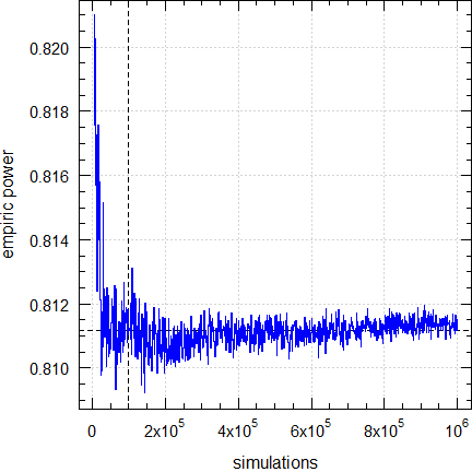
Dashed lines give the result (0.81116) obtained by the default (100,00 simulations).
Q: How reliable are the results?
A: As stated above an exact method doesn’t – and will never – exist. We can only compare the empiric power of the ABE-component to the exact one obtained bypower.TOST(). For an example see ‘Post hoc Power’ in the section about Dropouts.Q: Why give links to some references an HTTP-error 404 ‘Not found’?
A: I checked all URLs in April 2025. Contrary to us mere mortals who have to maintain a version control of documents, agencies don’t care. They change the structure of their websites (worst are the ones of the ANVISA and the WHO), don’t establish automatic redirects, rename or even delete files… Quod licet Iovi, non licet bovi
If you discover an error, please drop me a note at [email protected]..Q: I still have questions. How to proceed?
A: The preferred method is to register at the BEBA Forum and post your question in the category or (please read the Forum’s Policy first).
You can contact me at [email protected]. Be warned – I will charge you for anything beyond most basic questions.
top of section ↩︎ previous section ↩︎
Abbreviations
| Abbreviation | Meaning |
|---|---|
| (A)BE | (Average) Bioequivalence |
| ABEL | Average Bioequivalence with Expanding Limits |
| ASEAN | Association of Southeast Asian Nations |
| CI | \(\small{(1-2\,\alpha)}\) Confidence Interval |
| CL | Confidence Limit |
| \(\small{CV_\text{b}}\) | Between-subject Coefficient of Variation |
| \(\small{CV_\text{w}}\) | (Pooled) within-subject Coefficient of Variation |
| \(\small{CV_\text{wR},CV_\text{wT}}\) | Observed within-subject Coefficient of Variation of the Reference and Test product |
| EAC | East African Community |
| EEA | European Economic Area |
| EEU | Eurasian Economic Union |
| EMA | European Medicines Agency |
| EU | European Union |
| FDA | (U.S.) Food and Drug Administration |
| GCC | Gulf Cooperation Council |
| \(\small{H_0}\) | Null hypothesis (inequivalence) |
| \(\small{H_1}\) | Alternative hypothesis (equivalence) |
| HVD(P) | Highly Variable Drug (Product) |
| IBE | Individual Bioequivalence |
| ICH | International Council for Harmonisation |
| \(\small{k}\) | Regulatory constant (0.76) |
| NTID | Narrow Therapeutic Index Drug |
| PE | Point Estimate |
| \(\small{\text{R}}\) | Reference product |
| RSABE | Reference-Scaled Average Bioequivalence (FDA and China’s CDE) |
| SABE | Scaled Average Bioequivalence (ABEL and RSABE) |
| \(\small{s_\text{bR}^2,s_\text{bT}^2}\) | Observed between-subject variance of the Reference and Test product |
| \(\small{s_\text{wR},s_\text{wT}}\) | Observed within-subject standard deviation of the Reference and Test product |
| \(\small{s_\text{wR}^2,s_\text{wT}^2}\) | Observed within-subject variance of the Reference and Test product |
| \(\small{\text{T}}\) | Test product |
| TIE | Type I Error (patient’s risk) |
| TIIE | Type II Error (producer’s risk) |
| T/R | T/R-ratio (observed, PE) or assumed in sample size estimation |
| \(\small{uc}\) | Upper cap of expansion in ABEL |
| WHO | World Health Organization |
| \(\small{\alpha}\) | Nominal level of the test, probability of the Type I Error (patient’s risk) |
| \(\small{\beta}\) | Probability of the Type II Error (producer’s risk) |
| \(\small{\mu_\text{T}/\mu_\text{R},\theta_0}\) | True T/R-ratio |
| \(\small{\pi}\) | (Prospective) power, where \(\small{\pi=1-\beta}\) |
| \(\small{\sigma_\text{wR}}\) | True within-subject standard deviation of the Reference product |
| \(\small{\theta_1,\theta_2}\) | Fixed lower and upper limits of the acceptance range (generally 80.00 – 125.00%) |
| \(\small{\theta_{\text{s}_1},\theta_{\text{s}_2}}\) | Expanded lower and upper limits of the acceptance range \(\small{=100\exp(k\,\cdot s_\text{wR})}\); in the guidelines denoted as \(\small{\left\{\text{L},\text{U}\right\}}\) |
Licenses
 Helmut Schütz 2025
R, PowerTOST, and
pandoc GPL 3.0,
klippy MIT.
1st version March 23, 2021. Rendered April 10, 2025 11:37
CEST by rmarkdown via pandoc in 1.08 seconds.
Footnotes and References
FAX-machines.
Labes D, Schütz H, Lang B. PowerTOST: Power and Sample Size for (Bio)Equivalence Studies. Package version 1.5.6. 2024-03-18. CRAN.↩︎
Schütz H. Reference-Scaled Average Bioequivalence. 2024-02-29. CRAN.↩︎
Labes D, Schütz H, Lang B. Package ‘PowerTOST’. March 18, 2024. CRAN.↩︎
Some gastric resistant formulations of diclofenac are HVDPs, practically all topical formulations are HVDPs, whereas diclofenac itself is not a HVD (\(\small{CV_\text{w}}\) of a solution ~8%).↩︎
An inglorious counterexample: In the approval of dabigatran (the first univalent direct thrombin (IIa) inhibitor) the originator withheld information about severe bleeding events. Although it is highly variable, it is considered an NTID by the FDA and reference-scaling not acceptable. The study has to performed in a four period replicate design in order to allow a comparison of \(\small{s_\text{wT}}\) with \(\small{s_\text{wR}}\).↩︎
Tóthfalusi L, Endrényi L, García-Arieta A. Evaluation of bioequivalence for highly variable drugs with scaled average bioequivalence. Clin Pharmacokinet. 2009; 48(11): 725–43. doi:10.2165/11318040-000000000-00000.↩︎
ABEL is one variant of SABE. Another is Reference-Scaled Average Bioequivalence (RSABE), which is recommended by the FDA and China’s CDE. It is covered in another article.↩︎
GCC. Executive Directorate Of Benefits And Risks Evaluation. The GCC Guidelines for Bioequivalence. Version 2.4. 30/3/2016.
 Internet
Archive.↩︎
Internet
Archive.↩︎Final Concept Paper. M13: Bioequivalence for Immediate-Release Solid Oral Dosage Forms. Geneva. 19 June 2020. Endorsed 10 July 2020. Online.↩︎
ICH. Supplement to the “M13: Bioequivalence for Immediate-Release Solid Oral Dosage Forms” Concept Paper. Geneva. 13 December 2024. Online.↩︎
EMA, CHMP. Guideline on the Investigation of Bioequivalence. London. 20 January 2010. Online.↩︎
WHO, Essential Medicines and Health Products: Multisource (generic) pharmaceutical products: guidelines on registration requirements to establish interchangeability. WHO Technical Report Series, No. 1003, Annex 6. Geneva. 28 April 2017. Online↩︎
WHO/PQT: medicines. Guidance Document: Application of reference-scaled criteria for AUC in bioequivalence studies conducted for submission to PQT/MED. Geneva. 02 July 2021. Online.↩︎
Australian Government, Department of Health and Aged Care, TGA. International scientific guideline: Guideline on the investigation of bioequivalence. Canberra. Effective 16 June 2011. Online.↩︎
Shohin LE, Rozhdestvenkiy DA, Medvedev VYu, Komarow TN, Grebenkin DYu. Russia, Belarus & Kazakhstan. In: Kanfer I, editor. Bioequivalence Requirements in Various Global Jurisdictions. Charm: Springer; 2017. pp. 215–6.↩︎
EAC, Medicines and Food Safety Unit. Compendium of Medicines Evaluation and Registration for Medicine Regulation Harmonization in the East African Community, Part III: EAC Guidelines on Therapeutic Equivalence Requirements. Online.↩︎
ASEAN States Pharmaceutical Product Working Group. ASEAN Guideline for the Conduct of Bioequivalence Studies. Vientiane. March 2015. Online.↩︎
Shohin LE, Rozhdestvenkiy DA, Medvedev VYu, Komarow TN, Grebenkin DYu. Russia, Belarus & Kazakhstan. In: Kanfer I, editor. Bioequivalence Requirements in Various Global Jurisdictions. Charm: Springer; 2017. p. 207.↩︎
Eurasian Economic Commission. Regulations Conducting Bioequivalence Studies within the Framework of the Eurasian Economic Union. 3 November 2016, amended 15 February 2023. Online. [Russian]↩︎
Egyptian Drug Authority, Central Administration of Pharmaceutical Products. Egyptian Guidelines on Conducting Bioequivalence Studies for Marketing Authorization of Generic Products. Cairo. February 2017. Online.↩︎
New Zealand Medicines and Medical Devices Safety Authority. Guideline on the Regulation of Therapeutic Products in New Zealand. Part 6: Bioequivalence of medicines. Wellington. February 2018. Online.↩︎
Departamento Agencia Nacional de Medicamentos. Instituto de Salud Pública de Chile. Guia para La realización de estudios de biodisponibilidad comparativa en formas farmacéuticas sólidas de administración oral y acción sistémica. Santiago. December 2018. [Spanish]↩︎
ANVISA. Dispõe sobre os critérios para a condução de estudos de biodisponibilidade relativa/bioequivalência (BD/BE) e estudos farmacocinéticos. Brasilia. 17 August 2022. Online. [Portuguese]↩︎
Executive Board of the Health Ministers’ Council for GCC States. The GCC Guidelines for Bioequivalence. Version 3.1. 10 August 2022. Online.↩︎
Secretaría de Salud. Disposiciones para los Estudios de Bioequivalencia para Fármacos Altamente Variables. Ciudad de México. 24 January 2023. Online. [Spanish]↩︎
Health Canada. Guidance Document. Comparative Bioavailability Standards: Formulations Used for Systemic Effects. Ottawa. 08 June 2018. Online.↩︎
EMA, CHMP. Guideline on the pharmacokinetic and clinical evaluation of modified release dosage forms. London. 20 November 2014. Online.↩︎
Midha KK, Rawson MJ, Hubbard JW. Prescribability and switchability of highly variable drugs and drug products. J Contr Rel. 1999; 62(1-2): 33–40. doi:10.1016/s0168-3659(99)00050-4.↩︎
Labes D, Schütz H. Inflation of Type I Error in the Evaluation of Scaled Average Bioequivalence, and a Method for its Control. Pharm Res. 2016: 33(11); 2805–14. doi:10.1007/s11095-016-2006-1.↩︎
Schütz H, Labes D, Wolfsegger MJ. Critical Remarks on Reference-Scaled Average Bioequivalence. J Pharm Pharmaceut Sci. 2022; 25: 285–296. doi:10.18433/jpps32892.
 Open
Access.↩︎
Open
Access.↩︎Schütz H, Tomashevskiy M, Labes D. replicateBE: Average Bioequivalence with Expanding Limits (ABEL). Package version 1.1.3. 2022-05-02. CRAN.↩︎
Karalis V, Symillides M, Macheras P. On the leveling-off properties of the new bioequivalence limits for highly variable drugs of the EMA guideline. Europ J Pharm Sci. 2011; 44: 497–505. doi:10.1016/j.ejps.2011.09.008.↩︎
Commission of the European Communities, CPMP Working Party on Efficacy of Medicinal Products. Note for Guidance: Investigation of Bioavailability and Bioequivalence. Appendix III: Technical Aspects of Bioequivalence Statistics. Brussels. December 1991.↩︎
Commission of the European Communities, CPMP Working Party on Efficacy of Medicinal Products. Note for Guidance: Investigation of Bioavailability and Bioequivalence. June 1992.↩︎
Blume H, Mutschler E, editors. Bioäquivalenz. Qualitätsbewertung wirkstoffgleicher Fertigarzneimittel. Frankfurt / Main: Govi-Verlag; 6. Ergänzungslieferung 1996. [German]↩︎
EMA, CHMP EWP, Therapeutic Subgroup on Pharmacokinetics. Questions & Answers on the Bioavailability and Bioequivalence Guideline. London. 27 July 2006. Online.↩︎
MCC. Registration of Medicines. Biostudies. Pretoria. June 2015. Online.↩︎
League of Arab States, Higher Technical Committee for Arab Pharmaceutical Industry. Harmonised Arab Guideline on Bioequivalence of Generic Pharmaceutical Products. Cairo. March 2014. Online.↩︎
Shohin LE, Rozhdestvenkiy DA, Medvedev VYu, Komarow TN, Grebenkin DYu. Russia, Belarus & Kazakhstan. In: Kanfer I, editor. Bioequivalence Requirements in Various Global Jurisdictions. Charm: Springer; 2017. p. 222.↩︎
Of note, for NTIDs Health Canada’s limits are 90.0 – 112.0% and not 90.00 – 111.11% like in other jurisdictions. Guess the reason.↩︎
That’s contrary to ABE, where \(\small{CV_\text{w}}\) is an assumption as well.↩︎
Senn S. Guernsey McPearson’s Drug Development Dictionary. 21 April 2020. Online.↩︎
Hoenig JM, Heisey DM. The Abuse of Power: The Pervasive Fallacy of Power Calculations for Data Analysis. Am Stat. 2001; 55(1): 19–24. doi:10.1198/000313001300339897.
Open
Access.↩︎There is no statistical method to ‘correct’ for unequal carryover. It can only be avoided by design, i.e., a sufficiently long washout between periods. According to the guidelines subjects with pre-dose concentrations > 5% of their Cmax can by excluded from the comparison if stated in the protocol.↩︎
This is not always the case in ABEL. This issue is elaborated in another article.↩︎
Senn S. Statistical Issues in Drug Development. Chichester: John Wiley; 2nd ed. 2007.↩︎
Zhang P. A Simple Formula for Sample Size Calculation in Equivalence Studies. J Biopharm Stat. 2003; 13(3): 529–38. doi:10.1081/BIP-120022772.↩︎
Don’t be tempted to assume a ‘better’ T/R-ratio – even if based on a pilot or a previous study. It is a natural property of HVDPs that the T/R-ratio varies between studies. Don’t be overly optimistic!↩︎
Doyle AC. Adventures of Sherlock Holmes. Adventure I.—A Scandal in Bohemia. The Strand Magazine. 1891; 2(7): 63.↩︎
Schütz H. Sample Size Estimation in Bioequivalence. Evaluation. 2020-10-23. BEBA Forum. Vienna. 2020-10-23. Online.↩︎
Lenth RV. Two Sample-Size Practices that I Don’t Recommend. October 24, 2000. Online.↩︎
The only exception is
design = "2x2x3"(the full replicate with sequences TRT|RTR). Then the first element is for sequence TRT and the second for RTR.↩︎Quoting my late father: »If you believe, go to church.«↩︎
Molins E, Cobo E, Ocaña J. Two-Stage Designs Versus European Scaled Average Designs in Bioequivalence Studies for Highly Variable Drugs: Which to Choose? Stat Med. 2017; 36(30): 4777–88. doi:10.1002/sim.7452.↩︎
Berger RL, Hsu JC. Bioequivalence Trials, Intersection-Union Tests and Equivalence Confidence Sets. Stat Sci. 1996; 11(4): 283–302. JSTOR:2246021.↩︎
Zeng A. The TOST confidence intervals and the coverage probabilities with R simulation. March 14, 2014. Online.↩︎
The R Foundation for Statistical Computing. A Guidance Document for the Use of R in Regulated Clinical Trial Environments. Vienna. October 18, 2021. Online.↩︎
The R Foundation for Statistical Computing. R: Software Development Life Cycle. A Description of R’s Development, Testing, Release and Maintenance Processes. Vienna. October 18, 2021. Online.↩︎
FDA. General Principles of Software Validation; Final Guidance for Industry and FDA Staff. Rockville. January 11, 2002. Download.↩︎
FDA. Statistical Software Clarifying Statement. May 6, 2015. Online.↩︎
WHO. Guidance for organizations performing in vivo bioequivalence studies. Technical Report Series No. 996, Annex 9. Section 4. Geneva. May 2016. Online.↩︎
EMA, GCP IWG. Guideline on computerised systems and electronic data in clinical trials. Amsterdam. 9 March 2023. Online.↩︎
Tóthfalusi L, Endrényi L. Sample Sizes for Designing Bioequivalence Studies for Highly Variable Drugs. J Pharm Pharmacol Sci. 2012; 15(1): 73–84. doi:10.18433/j3z88f.
Open
Access.↩︎User ‘BEQool’. ABEL is a framework (decision scheme). BEBA Forum. Vienna. 2024-01-30. Online.↩︎