
Sample Size Estimation for Equivalence Studies of NTIDs
(U.S. FDA, China CDE)
Helmut Schütz
June 21, 2023
Consider allowing JavaScript. Otherwise, you have to be proficient in
reading  since formulas
will not be rendered. Furthermore, the table of contents in the left
column for navigation will not be available and code-folding not
supported. Sorry for the inconvenience.
since formulas
will not be rendered. Furthermore, the table of contents in the left
column for navigation will not be available and code-folding not
supported. Sorry for the inconvenience.
Examples in this article were generated with
 4.3.1
by the package
4.3.1
by the package PowerTOST.1
See also the README on GitHub for an overview and the Online manual2 for details.
- The right-hand badges give the respective section’s ‘level’.
- Basics about sample size methodology – requiring no or only limited statistical expertise.
- These sections are the most important ones. They are – hopefully – easily comprehensible even for novices.
- A somewhat higher knowledge of statistics and/or R is required. May be skipped or reserved for a later reading.
- An advanced knowledge of statistics and/or R is required. Not recommended for beginners in particular.
- Click to show / hide R code.
- To copy R code to the clipboard click on
the icon
 in the top left corner.
| Abbreviation | Meaning |
|---|---|
| (A)BE | (Average) Bioequivalence |
| \(\small{CV_\textrm{b}}\) | Between-subject Coefficient of Variation |
| \(\small{CV_\textrm{w}}\) | Within-subject Coefficient of Variation |
| \(\small{CV_\textrm{wT}}\), \(\small{CV_\textrm{wR}}\) | Within-subject Coefficient of Variation of the Test and Reference drug |
| \(\small{H_0}\) | Null hypothesis |
| \(\small{H_1}\) | Alternative hypothesis (also \(\small{H_\textrm{a}}\)) |
| NTI(D) | Narrow Therapeutic Index (Drug) |
| RSABE | Reference-scaled Average Bioequivalence |
| \(\small{s_0}\) | Switching standard deviation (0.10) |
| SABE | Scaled Average Bioequivalence |
| \(\small{s_\textrm{wT}}\), \(\small{s_\textrm{wR}}\) | Within-subject standard deviation of the Test and Reference drug |
| \(\small{s_\textrm{wT}^2}\), \(\small{s_\textrm{wR}^2}\) | Within-subject variance of the Test and Reference drug |
| \(\small{\theta_\textrm{s}}\) | Regulatory constant (1.053605…) |
| \(\small{\left\{\theta_{\textrm{s}_1},\theta_{\textrm{s}_2}\right\}}\) | Scaled limits |
Introduction
What is Reference-scaled Average Bioequivalence for Narrow Therapeutic Index Drugs?
For background about inferential statistics see this article.
Narrow Therapeutic Index (NTI) Drugs are defined as those where small differences in dose or blood concentration may lead to serious therapeutic failures and/or adverse drug reactions that are life-threatening or result in persistent or significant disability or incapacity.
- The conventional ‘clinically relevant difference’ Δ of 20% (leading to the limits of 80.00 – 125.00% in Average Bioequivalence (ABE) is considered liberal.
- Hence, a more strict Δ of < 20% was proposed. A natural approach is to scale (narrow) the limits based on the within-subject variability of the reference product σwR.3 4 5 6 7
The conventional confidence interval inclusion approach of ABE \[\begin{matrix}\tag{1} \theta_1=1-\Delta,\theta_2=\left(1-\Delta\right)^{-1}\\ H_0:\;\frac{\mu_\textrm{T}}{\mu_\textrm{R}}\ni\left\{\theta_1,\,\theta_2\right\}\;vs\;H_1:\;\theta_1<\frac{\mu_\textrm{T}}{\mu_\textrm{R}}<\theta_2, \end{matrix}\] where \(\small{H_0}\) is the null hypothesis of inequivalence and \(\small{H_1}\) the alternative hypothesis, \(\small{\theta_1}\) and \(\small{\theta_2}\) are the fixed lower and upper limits of the acceptance range, and \(\small{\mu_\textrm{T}}\) are the geometric least squares means of \(\small{\textrm{T}}\) and \(\small{\textrm{R}}\), respectively, is in Scaled Average Bioequivalence (SABE) modified to \[H_0:\;\frac{\mu_\textrm{T}}{\mu_\textrm{R}}\Big{/}\sigma_\textrm{wR}\ni\left\{\theta_{\textrm{s}_1},\,\theta_{\textrm{s}_2}\right\}\;vs\;H_1:\;\theta_{\textrm{s}_1}<\frac{\mu_\textrm{T}}{\mu_\textrm{R}}\Big{/}\sigma_\textrm{wR}<\theta_{\textrm{s}_2},\tag{2}\] where \(\small{\sigma_\textrm{wR}}\) is the standard deviation of the reference and the scaled limits \(\small{\left\{\theta_{\textrm{s}_1},\,\theta_{\textrm{s}_2}\right\}}\) of the acceptance range depend on conditions given by the agency. NB, the guidance of China’s CDE is essentially a 1:1 translation of the FDA’s guidances.
The hypotheses in the applicable linearized model are \[H_0:(\mu_\textrm{T}/\mu_\textrm{R})^2-\theta_\textrm{s}\cdot s_\textrm{wR}^{2}>0\:vs\:H_1:(\mu_\textrm{T}/\mu_\textrm{R})^2-\theta_\textrm{s}\cdot s_\textrm{wR}^{2}\leq 0\tag{3}\]
Note that in other jurisdictions fixed narrower limits (i.e., 90.00 – 111.11% based on Δ 10%) are recommended. The applicant is free to select a conventional 2×2×2 crossover or a replicate design.
In order to apply RSABE the study has to be performed in a full replicate design (i.e., both the test and reference drug have to be administered twice). The FDA recommends a two-sequence four-period design (TRTR|RTRT), although full replicate designs with only three periods (TRT|RTR or TTR|RRT) would serve the purpose as well.
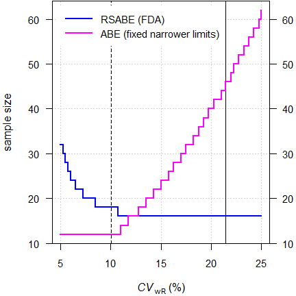
Fig. 1 Sample sizes for RSABE
and ABE with fixed narrower limits.
TRTR|RTRT-design, assumed
T/R-ratio 0.975 targeted at ≥ 80% power,
homoscedasticity (\(\small{s_\textrm{wT}^2=s_\textrm{wR}^2}\)).
The approach given in the
FDA’s guidances
hinges on the estimated standard deviation of the reference treatment
\(\small{s_{\textrm{wR}}}\) to decide
upon the degree of narrowing.
Furthermore, \(\small{s_\textrm{wT}/s_\textrm{wR}\leq2.5}\)
and the 90% Confidence Interval (CI) has to lie entirely within 80.00 –
125.00%.
Based on the switching standard deviation \(\small{s_0=0.10}\) we get the regulatory constant \(\small{\theta_\textrm{s}=\frac{\log_{e}(1/0.9)}{s_0}=1.053605\ldots}\) and the scaled limits \(\small{\left\{\theta_{\textrm{s}_1},\theta_{\textrm{s}_2}\right\}=100\,\exp(\mp1.053605\cdot s_{\textrm{wR}})}\).
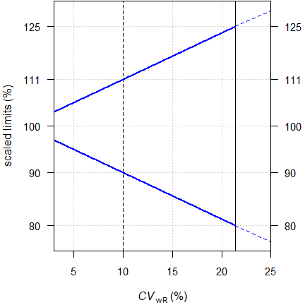
Fig. 2 Scaled limits.
Dashed
line at the switching condition \(\small{s_0}\) (\(\small{CV_0\approx10.02505\%}\))
and
solid line at the ‘implied’ upper cap (\(\small{CV_\textrm{wR}\approx
21.4188\%}\)).
At \(\small{s_0=0.10}\) (\(\small{CV_0\approx10.02505\%}\)) the scaled limits are \(\small{90.00-\dot{1}11.11\%}\). There is an ‘implied’ upper cap of scaling at \(\small{CV_\textrm{wR}\approx 21.4188\%}\). Otherwise, scaled limits would be wider than \(\small{80.00-125.00\%}\) (the blue dashed lines in Fig. 2). Practically the upper cap is not used (like in ABEL for HVDs) but additionally conventional ABE assessed.
Since the applicability of this approach depends on the realized values of \(\small{s_\textrm{wT}}\) and \(\small{s_\textrm{wR}}\) in the particular study – which are naturally unknown beforehand – analytical solutions for power (and hence, the sample size) do not exist.
Therefore, extensive simulations of potential combinations have to be employed.
Preliminaries
A basic knowledge of R is
required. To run the scripts at least version 1.2.8 (2015-07-10) of
PowerTOST is required and 1.5.3 (2021-01-18) suggested. Any
version of R would likely do, though the
current release of PowerTOST was only tested with version
4.1.3 (2022-03-10) and later.
All scripts were run on a Xeon E3-1245v3 @ 3.40GHz (1/4 cores) 16GB RAM
with R 4.3.1 on Windows 7 build 7601, Service
Pack 1, Universal C Runtime 10.0.10240.16390.
Note that in all functions of PowerTOST the arguments
(say, the assumed T/R-ratio theta0, the assumed coefficient
of variation CV, etc.) have to be given as ratios and not
in percent.
sampleN.NTID() gives balanced sequences (i.e.,
an equal number of subjects is allocated to all sequences). Furthermore,
the estimated sample size is the total number of subjects.
All examples deal with studies where the response variables likely follow a lognormal distribution, i.e., we assume a multiplicative model (ratios instead of differences). We work with \(\small{\log_{e}}\)-transformed data in order to allow analysis by the t-test (requiring differences).
Terminology
It may sound picky but ‘sample size calculation’ (as used in most guidelines and alas, in some publications and textbooks) is sloppy terminology. In order to get prospective power (and hence, a sample size), we need five values:
- The level of the test (in BE commonly 0.05),
- the (potentially) narrowed BE-margin,
- the desired (or target) power,
- the variance (commonly expressed as a coefficient of variation), and
- the deviation of the test from the reference treatment,
where
- is fixed by the agency,
- depends on the observed9 CVwR (which is unknown beforehand),
- is set by the sponsor (commonly to 0.80 – 0.90),
- is an uncertain assumption,
- is an uncertain assumption.
In other words, obtaining a sample size is not an exact calculation like \(\small{2\times2=4}\) but always just an estimation.
“Power Calculation – A guess masquerading as mathematics.
Of note, it is extremely unlikely that all assumptions will be exactly realized in a particular study. Hence, calculating retrospective (a.k.a. post hoc, a posteriori) power is not only futile but plain nonsense.11
Since generally the within-subject variability \(\small{CV_\textrm{w}}\) is smaller than the
between-subject variability \(\small{CV_\textrm{b}}\), crossover studies
are so popular.
Of note, there is no relationship between \(\small{CV_\textrm{w}}\) and \(\small{CV_\textrm{b}}\). An example are
drugs which are subjected to polymorphic metabolism. For these drugs
\(\small{CV_\textrm{w}\ll
CV_\textrm{b}}\).
Furthermore, the drugs’ within-subject variability may be unequal
(i.e., \(\small{s_{\textrm{wT}}^{2}\neq
s_{\textrm{wR}}^{2}}\)). For details see the section about Heteroscedasticity.
It is a prerequisite that no (unequal) carryover from one period to the next exists. Only then the comparison of treatments will be unbiased.12 Carryover is elaborated in another article.
Power → Sample size
The sample size cannot be
directly estimated, in
SABE only power
simulated
for an already given sample size based on
assumptions.
“Power. That which statisticians are always calculating but never have.
Let’s start with PowerTOST.
library(PowerTOST) # attach it to run the examples| Argument | Default | Meaning |
|---|---|---|
alpha
|
0.05
|
Nominal level of the test. |
targetpower
|
0.80
|
Target (desired) power. |
theta0
|
0.975
|
Assumed T/R-ratio. |
theta1
|
0.80
|
Lower acceptance limit in ABE. |
theta2
|
1.25
|
Upper acceptance limit in ABE. |
design
|
"2x2x4"
|
Treatments × Sequences × Periods. |
nsims
|
1e05
|
Number of simulations (fewer are not recommended). |
print
|
TRUE
|
Output to the console. |
details
|
TRUE
|
Show regulatory settings and sample size search. |
setseed
|
TRUE
|
Set a fixed seed (recommended for reproducibility). |
The sample size functions of PowerTOST use a
modification of Zhang’s method15 based on the large sample approximation
as the starting value of the iterations.
# Note that theta0 = 0.975, targetpower = 0.80, and
# design = "2x2x4" are defaults
sampleN.NTID(CV = 0.125, details = TRUE)
#
# +++++++++++ FDA method for NTIDs ++++++++++++
# Sample size estimation
# ---------------------------------------------
# Study design: 2x2x4 (TRTR|RTRT)
# log-transformed data (multiplicative model)
# 1e+05 studies for each step simulated.
#
# alpha = 0.05, target power = 0.8
# CVw(T) = 0.125, CVw(R) = 0.125
# True ratio = 0.975
# ABE limits = 0.8 ... 1.25
# Implied scABEL = 0.8771 ... 1.1402
# Regulatory settings: FDA
# - Regulatory const. = 1.053605
# - 'CVcap' = 0.2142
#
# Sample size search
# n power
# 14 0.752830
# 16 0.822780Examples
Throughout the examples I’m referring to studies in a single center – not multiple groups within them or multicenter studies. That’s another cup of tea.
A Simple Case
We assume a CV of 0.125, a T/R-ratio of 0.975, a target a power of 0.80, and want to perform the study in a 2-sequence 4-period full replicate study (TRTR|RTRT).
Since theta0 = 0.975,16 17
targetpower = 0.80, and design = "2x2x4" are
defaults of the function, we don’t have to give
them explicitely. As usual in bioequivalence, alpha = 0.05
is employed (we will assess the study by a \(\small{100\,(1-2\,\alpha)=90\%}\)
CI). Hence, you need to specify
only the CV (assuming \(\small{CV_\textrm{wT}=CV_\textrm{wR}}\)).
To shorten the output, use the argument
details = FALSE.
sampleN.NTID(CV = 0.125, details = FALSE)#
# +++++++++++ FDA method for NTIDs ++++++++++++
# Sample size estimation
# ---------------------------------------------
# Study design: 2x2x4 (TRTR|RTRT)
# log-transformed data (multiplicative model)
# 1e+05 studies for each step simulated.
#
# alpha = 0.05, target power = 0.8
# CVw(T) = 0.125, CVw(R) = 0.125
# True ratio = 0.975
# ABE limits = 0.8 ... 1.25
# Regulatory settings: FDA
#
# Sample size
# n power
# 16 0.822780Sometimes we are not interested in the entire output and want to use
only a part of the results in subsequent calculations. We can suppress
the output by stating the additional argument print = FALSE
and assign the result to a data frame (here named x).
x <- sampleN.NTID(CV = 0.125, details = FALSE, print = FALSE)Although you could access the elements by the number of the
column(s), I don’t recommend that, since in other functions of
PowerTOST these numbers are different and hence, difficult
to remember.
Let’s retrieve the column names of x:
names(x)
#  [1] "Design"         "alpha"          "CVwT"           "CVwR"
#  [5] "theta0"         "theta1"         "theta2"         "Sample size"
#  [9] "Achieved power" "Target power"   "nlast"
Now we can access the elements of x by their names. Note
that double square brackets [["foo"]] have to be used,
where "foo" is the name of the element.
x[["Sample size"]]
# [1] 16
x[["Achieved power"]]
# [1] 0.82278
If you insist in accessing elements by column-numbers, use single
square brackets [bar], where bar is the
respective number. You could also access multiple columns,
e.g., [foo:bar] or even as a vector
[c(foo, bar:baz)].
x[8:9]
#   Sample size Achieved power
# 1          16        0.82278
x[c(4, 8:9)]
#    CVwR Sample size Achieved power
# 1 0.125          16        0.82278
With 16 subjects (eight per sequence) we achieve the power we desire.
What will happen if we have one dropout?
power.NTID(CV = 0.125, n = x[["Sample size"]] - 1)# Unbalanced design. n(i)=8/7 assumed.# [1] 0.78896Slightly below the 0.80 we desire.
Since dropouts are common, it makes sense to include / dose more subjects in order to end up with a number of eligible subjects which is not lower than our initial estimate.
Let us explore that in the next section.
Dropouts
We define two supportive functions:
- Provide equally sized sequences, i.e., any total sample
size
nwill be rounded up to achieve balance.
balance <- function(n, n.seq) {
  return(as.integer(n.seq * (n %/% n.seq + as.logical(n %% n.seq))))
}- Provide the adjusted sample size based on the original sample size
nand the anticipated droput-ratedo.rate.
nadj <- function(n, do.rate, n.seq) {
  return(as.integer(balance(n / (1 - do.rate), n.seq)))
}
In order to come up with a suggestion we have to anticipate a (realistic!) dropout rate. Note that this not the job of the statistician; ask the Principal Investigator.
“It is a capital mistake to theorize before one has data. Insensibly one begins to twist facts to suit theories, instead of theories to suit facts.
Dropout-rate
The dropout-rate is calculated from the eligible and
dosed subjects
or simply \[\begin{equation}\tag{4}
do.rate=1-n_\textrm{eligible}/n_\textrm{dosed}
\end{equation}\] Of course, we know it only after the
study was performed.
By substituting \(n_\textrm{eligible}\) with the estimated sample size \(n\), providing an anticipated dropout-rate and rearrangement to find the adjusted number of dosed subjects \(n_\textrm{adj}\), we should use \[\begin{equation}\tag{5} n_\textrm{adj}=\;\upharpoonleft n\,/\,(1-do.rate) \end{equation}\] where \(\upharpoonleft\) denotes eventual rounding up to obtain a multiple of the number of sequences as implemented in the functions above.
An all too common mistake is to increase the estimated sample size \(n\) by the dropout-rate according to \[\begin{equation}\tag{6} n_\textrm{adj}=\;\upharpoonleft n\times(1+do.rate) \end{equation}\] If you used \(\small{(6)}\) in the past – you are not alone. In a small survey a whopping 29% of respondents reported to use it.19 Consider changing your routine.
“There are no routine statistical questions, only questionable statistical routines.
Adjusted Sample Size
In the following I specified more arguments to make the function more
flexible.
Note that I wrapped the function power.RSABE() in
suppressMessages(). Otherwise, the function will throw for
any sample size with unbalanced sequences (odd for a 4-period
design and even for a 3-period design) a message telling us
that the design is unbalanced. Well, we know that.
CV      <- 0.125 # within-subject CV
target  <- 0.80  # target (desired) power
theta0  <- 0.975 # assumed T/R-ratio
design  <- "2x2x4"
do.rate <- 0.15  # anticipated dropout-rate 15%
                 # might be relatively high
                 # due to the 4 periods
n.seq   <- as.integer(substr(design, 3, 3))
d.f     <- sampleN.NTID(CV = CV, theta0 = theta0,
                        targetpower = target,
                        design = design,
                        details = FALSE,
                        print = FALSE)
# calculate the adjusted sample size
n.adj   <- nadj(d.f[["Sample size"]], do.rate, n.seq)
# (decreasing) vector of eligible subjects
n.elig  <- n.adj:d.f[["Sample size"]]
info    <- paste0("Assumed CV              : ",
                  CV,
                  "\nAssumed T/R ratio       : ",
                  theta0,
                  "\nTarget (desired) power  : ",
                  target,
                  "\nAnticipated dropout-rate: ",
                  do.rate,
                  "\nEstimated sample size   : ",
                  d.f[["Sample size"]], " (",
                  d.f[["Sample size"]]/n.seq, "/sequence)",
                  "\nAchieved power          : ",
                  signif(x[["Achieved power"]], 4),
                  "\nAdjusted sample size    : ",
                  n.adj, " (",  n.adj/n.seq, "/sequence)",
                  "\n\n")
# explore the potential outcome for
# an increasing number of dropouts
do.act <- signif((n.adj - n.elig) / n.adj, 4)
d.f     <- data.frame(dosed    = n.adj,
                      eligible = n.elig,
                      dropouts = n.adj - n.elig,
                      do.act   = do.act,
                      power    = NA_real_)
for (i in 1:nrow(d.f)) {
  d.f$power[i] <- suppressMessages(
                    power.NTID(CV = CV,
                               theta0 = theta0,
                               design = design,
                               n = d.f$eligible[i]))
}
cat(info)
print(round(d.f, 4), row.names = FALSE)
# Assumed CV : 0.125
# Assumed T/R ratio : 0.975
# Target (desired) power : 0.8
# Anticipated dropout-rate: 0.15
# Estimated sample size : 16 (8/sequence)
# Achieved power : 0.8228
# Adjusted sample size : 20 (10/sequence)
#
# dosed eligible dropouts do.act power
# 20 20 0 0.00 0.9091
# 20 19 1 0.05 0.8904
# 20 18 2 0.10 0.8734
# 20 17 3 0.15 0.8485
# 20 16 4 0.20 0.8228In the worst case (four dropouts) we end up with the originally estimated sample size of 16 subjects. Power preserved, mission accomplished. If we have fewer dropouts, splendid – we gain power.
Post hoc Power
As said in the preliminaries, calculating post hoc power is futile.
“There is simple intuition behind results like these: If my car made it to the top of the hill, then it is powerful enough to climb that hill; if it didn’t, then it obviously isn’t powerful enough. Retrospective power is an obvious answer to a rather uninteresting question. A more meaningful question is to ask whether the car is powerful enough to climb a particular hill never climbed before; or whether a different car can climb that new hill. Such questions are prospective, not retrospective.
However, sometimes we are interested in it for planning the next study.
If you give a total sample size n which is not a
multiple of the number of sequences, power.NTID() will try
to keep sequences as balanced as possible and show in a message how that
was done.
n.act <- 17
signif(power.NTID(CV = 0.125, n = n.act), 6)
# Unbalanced design. n(i)=9/8 assumed.# [1] 0.84853Say, our study was more unbalanced. Let us assume that we dosed 20
subjects, the total number of subjects was also 17 but all dropouts
occured in one sequence (unlikely though possible).
Instead of the total sample size n we can give the number
of subjects in each sequence as a vector (the order is generally21 not
relevant, i.e., it does not matter which element refers to
which sequence).
By setting details = TRUE we can retrieve the components
of the simulations (probability to pass each test).
design   <- "2x2x4"
CV       <- 0.125
n.adj    <- 20
n.act    <- 17
n.s1     <- n.adj / 2
n.s2     <- n.act - n.s1
theta0   <- 0.975
post.hoc <- suppressMessages(
              power.NTID(CV  = CV,
                         n = c(n.s1, n.s2),
                         theta0 = theta0,
                         design = design,
                         details = TRUE))
ABE.xact <- power.TOST(CV = CV,
                       n = c(n.s1, n.s2),
                       theta0 = theta0,
                       robust = TRUE, # mixed-effects model's df
                       design = design)
sig.dig  <- nchar(as.character(n.adj))
fmt      <- paste0("%", sig.dig, ".0f (%",
                   sig.dig, ".0f dropouts)")
cat(paste0("Dosed subjects : ", sprintf("%2.0f", n.adj),
           "\nEligible       : ",
           sprintf(fmt, n.act, n.adj - n.act),
           "\n  Sequence 1   : ",
           sprintf(fmt, n.s1, n.adj / 2 - n.s1),
           "\n  Sequence 1   : ",
           sprintf(fmt, n.s2, n.adj / 2 - n.s2),
           "\nPower (overall):  ",
           sprintf("%.5f", post.hoc[1]),
           "\n  p(SABE)      :  ",
           sprintf("%.5f", post.hoc[3]),
           "\n  p(s-ratio)   :  ",
           sprintf("%.5f", post.hoc[2]),
           "\n  p(ABE)       :  ",
           sprintf("%.5f", post.hoc[4]),
           "\n  p(ABE) exact :  ",
           sprintf("%.5f", ABE.xact), "\n"))
# Dosed subjects : 20
# Eligible : 17 ( 3 dropouts)
# Sequence 1 : 10 ( 0 dropouts)
# Sequence 1 : 7 ( 3 dropouts)
# Power (overall): 0.84227
# p(SABE) : 1.00000
# p(s-ratio) : 0.86233
# p(ABE) : 0.96330
# p(ABE) exact : 1.00000The components of overall power are:
p(SABE)is the probability of passing SABE (bound ≤ 0) acc. to (3).p(s-ratio)is the probability of passing the ratio test (upper confidence limit of σwT/σwR ≤ 2.5).p(ABE)is the probability of passing conventional ABE (90% CI within 80.00 – 125.00%) acc. to (1).p(ABE) exactis the probability of passing ABE obtained bypower.TOST(), i.e., without simulations.
Of course, in a particular study you will provide the numbers in the
n vector directly.
Lost in Assumptions
The CV and the T/R-ratio are only assumptions.
Whatever their origin might be (literature, previous studies) they carry
some degree of uncertainty. Hence, believing22 that they are the
true ones may be risky.
Some statisticians call that the ‘Carved-in-Stone’ approach.
Say, we performed a pilot study in twelve subjects and estimated the CV as 0.125.
A two-sided confidence interval of the CV can be obtained via the \(\small{\chi^2}\)-distribution of its error variance \(\small{\sigma^2}\) with \(\small{n-2}\) degrees of freedom. \[\eqalign{\tag{7} s^2&=\log_{e}(CV^2+1)\\ L=\frac{(n-1)\,s^2}{\chi_{\alpha/2,\,n-2}^{2}}&\leq\sigma^2\leq\frac{(n-1)\,s^2}{\chi_{1-\alpha/2,\,n-2}^{2}}=U\\ \left\{lower\;CL,\;upper\;CL\right\}&=\left\{\sqrt{\exp(L)-1},\sqrt{\exp(U)-1}\right\} }\]
Let’s calculate the 95% confidence interval of the CV to get an idea.
m  <- 12 # pilot study
ci <- CVCL(CV = 0.125, df = m - 2,
           side = "2-sided", alpha = 0.05)
signif(ci, 4)
# lower CL upper CL
# 0.08717 0.22120Surprised? Although 0.125 is the best estimate for planning the next study, there is no guarantee that we will get exactly the same outcome. Since the \(\small{\chi^2}\)-distribution is skewed to the right, it is more likely to get a higher CV than a lower one in the planned study.
If we plan the study based on 0.125, we would opt for 16 subjects
like in the example before (not adjusted for the dropout-rate).
If the CV will be lower, we loose power (narrower limits). But
what if it will be higher? Depends. Since we have to narrow the limits
less, we gain power. But how much?
Let’s explore what might happen at the confidence limits of the CV.
m    <- 12
ci   <- CVCL(CV = 0.125, df = m - 2,
             side = "2-sided", alpha = 0.05)
n    <- 16
comp <- data.frame(CV = c(ci[["lower CL"]], 0.125,
                          ci[["upper CL"]]),
                          power = NA_real_)
for (i in 1:nrow(comp)) {
  comp$power[i] <- power.NTID(CV = comp$CV[i], n = n)
}
comp[, 1] <- signif(comp[, 1], 4)
comp[, 2] <- signif(comp[, 2], 6)
print(comp, row.names = FALSE)
# CV power
# 0.08717 0.75885
# 0.12500 0.82278
# 0.22120 0.85300What can we do? The larger the previous study was, the larger the degrees of freedom and hence, the narrower the confidence interval of the CV. In simple terms: The estimate is more certain. On the other hand, it also means that very small pilot studies are practically useless. What happens when we plan the study based on the confidence interval of the CV?
m               <- seq(6, 12, 2)
d.f             <- data.frame(n.pilot = m, CV = 0.125,
                              l = NA_real_, u = NA_real_,
                              n.low = NA_integer_, n.CV = NA_integer_,
                              n.hi = NA_integer_)
for (i in 1:nrow(d.f)) {
  d.f[i, 3:4] <- CVCL(CV = 0.125, df = m[i] - 2,
                     side = "2-sided", alpha = 0.05)
  d.f[i, 5] <- sampleN.NTID(CV = d.f$l[i], details = FALSE,
                            print = FALSE)[["Sample size"]]
  d.f[i, 6] <- sampleN.NTID(CV = 0.125, details = FALSE,
                            print = FALSE)[["Sample size"]]
  d.f[i, 7] <- sampleN.NTID(CV = d.f$u[i], details = FALSE,
                            print = FALSE)[["Sample size"]]
}

d.f[, 3:4]      <- signif(d.f[, 3:4], 4)
names(d.f)[3:4] <- c("lower CL", "upper CL")
print(d.f, row.names = FALSE)
# n.pilot CV lower CL upper CL n.low n.CV n.hi
# 6 0.125 0.07471 0.3696 20 16 26
# 8 0.125 0.08037 0.2794 20 16 18
# 10 0.125 0.08425 0.2420 18 16 16
# 12 0.125 0.08717 0.2212 18 16 16Small pilot studies are practically useless.
Furthermore, we don’t know where the true T/R-ratio lies but we can calculate the lower 95% confidence limit of the pilot study’s point estimate to get an idea about a worst case. Say, it was 0.975.
m      <- 12
CV     <- 0.125
pe     <- 0.975
ci     <- round(CI.BE(CV = CV, pe = pe, n = m,
                      design = "2x2x4"), 4)
if (pe <= 1) {
  cl <- ci[["lower"]]
} else {
  cl <- ci[["upper"]]
}
print(cl)
# [1] 0.9174We must not forget the ratio-test comparing the drugs’ within-subject standard deviations. Explore the impact of different CVs and a relatively 2.5% lower T/R-ratio on power for the given sample size.
n       <- 16
CV      <- 0.125
ratio   <- seq(1, 2, 0.5) # variance ratio (T/R)
theta0  <- 0.975
r_const <- -log(0.90) / 0.1
comp1   <- data.frame(CVwT = CVp2CV(0.125, ratio)[, 1],
                      CVwR = CVp2CV(0.125, ratio)[, 2],
                      s.ratio.CL =  NA_real_,
                      L = NA_real_, U = NA_real_,
                      power = NA_real_, SABE = NA_real_,
                      s.ratio = NA_real_)
comp2  <- data.frame(CV = CV, theta0 = c(theta0, theta0 * 0.975),
                     power = NA_real_)
for (i in seq_along(ratio)) {
  comp1$s.ratio.CL[i] <- CV2se(comp1$CVwT[i])/CV2se(comp1$CVwR[i]) /
                         sqrt(qf(1-0.1/2, df1 = n -2 , df2 = n -2,
                                 lower.tail = FALSE))
  comp1[i, 4:5] <- round(100 * exp(c(-1, +1) *
                                   r_const * CV2se(comp1$CVwR[i])), 2)
  tmp <- suppressMessages(
           power.NTID(CV = c(comp1$CVwT[i], comp1$CVwR[i]),
                      theta0 = theta0, n = n, details = TRUE))
  comp1$power[i]   <- tmp[["p(BE)"]]
  comp1$SABE[i]    <- tmp[["p(BE-sABEc)"]]
  comp1$s.ratio[i] <- tmp[["p(BE-sratio)"]]
}
comp1 <- signif(comp1, 5)
names(comp1)[7:8] <- c("p(SABE)", "p(s-ratio)")
for (i in 1:2) {
  comp2$power[i] <- power.NTID(CV = CV, theta0 = comp2$theta0[i],
                               n = n)
}
comp2 <- signif(comp2, 5)
print(comp1, row.names = FALSE)
print(comp2, row.names = FALSE)
# CVwT CVwR s.ratio.CL L U power p(SABE) p(s-ratio)
# 0.12500 0.12500 1.5760 87.71 114.02 0.82278 0.84869 0.95128
# 0.13704 0.11172 1.9302 88.93 112.45 0.67124 0.76335 0.82792
# 0.14452 0.10193 2.2288 89.84 111.31 0.50581 0.67983 0.66365
# CV theta0 power
# 0.125 0.97500 0.82278
# 0.125 0.95062 0.64342If \(\small{CV_\textrm{wT}>CV_\textrm{wR}}\)
(with \(\small{CV_\textrm{w}=\textrm{const}=0.125}\))
we are in trouble. The scaled limits get narrower and the impact of the
ratio-test becomes increasingly important. With \(\small{\sigma_\textrm{wT}^2/\sigma_\textrm{wR}^2=2}\)
the upper confidence limit of \(\small{s_\textrm{wT}/s_\textrm{wR}}\) is
with ≈2.23 already close to the limit of 2.5.
If the T/R-ratio gets even just a little worse, the impact on power is
substantial.
Essentially this leads to the murky waters of prospective power and sensitivity
analyses.
An appetizer to show the maximum deviations (CV, T/R-ratio and
decreased sample size due to dropouts) which give still a minimum
acceptable power of ≥ 0.70:
CV       <- 0.125
theta0   <- 0.975
target   <- 0.80
minpower <- 0.70
pa       <- pa.NTID(CV = CV, theta0 = theta0,
                    targetpower = target,
                    minpower = minpower)
change.CV     <- 100*(tail(pa$paCV[["CV"]], 1) -
                      pa$plan[["CVwR"]]) /
                      pa$plan[["CVwR"]]
change.theta0 <- 100*(head(pa$paGMR$theta0, 1) -
                      pa$plan$theta0) /
                      pa$plan[["theta0"]]
change.n      <- 100*(tail(pa$paN[["N"]], 1) -
                      pa$plan[["Sample size"]]) /
                      pa$plan[["Sample size"]]
comp     <- data.frame(parameter = c("CV", "theta0", "n"),
                       change = c(change.CV,
                                  change.theta0,
                                  change.n))
comp$change <- sprintf("%+.2f%%", comp$change)
names(comp)[2] <- "relative change"
print(pa, plotit = FALSE)
print(comp, row.names = FALSE)
# Sample size plan NTID
# Design alpha CVwT CVwR theta0 theta1 theta2 Sample size
# 2x2x4 0.05 0.125 0.125 0.975 0.8 1.25 16
# Achieved power Target power
# 0.82278 0.8
#
# Power analysis
# CV, theta0 and number of subjects leading to min. acceptable power of ~0.7:
# CV = (0.0716, 0.3059), theta0= 0.9569
# n = 13 (power= 0.7064)
#
# parameter relative change
# CV +144.76%
# theta0 -1.86%
# n -18.75%Confirms what we have seen above. As expected, the method is extremely robust to changes in the CV. The sample size is also not very sensitive; many overrate the impact of dropouts on power. As usual in bioequivalence, changes in the T/R-ratio hurt most.
Heteroscedasticity
Since a comparison of \(\small{s_\textrm{wT}}\) with \(\small{s_\textrm{wR}}\) is mandatory,
already pilot studies have to be performed in one of the fully
replicated designs. If you are concerned about dropouts or the
bioanalytical method requires large sample volumes, opt for one of the
2-sequence 3-period designs (TRT|RTR or TRR|RTT).
Since pharmaceutical technology – hopefully – improves, it is not
uncommon that \(\small{s_\textrm{wT}<s_\textrm{wR}}\).
If this is the case, you get an incentive in the sample size of the
pivotal study; scaling the limits is based on \(\small{s_\textrm{wR}}\) but the 90%
CI in the
ABE-component on the
(pooled) \(\small{s_\textrm{w}^{2}}\).
Furthermore, the probability to pass the ratio-test increases.
\[\eqalign{\tag{8} s_\textrm{wT}^{2}&=\log_{e}(CV_\textrm{wT}^{2}+1)\\ s_\textrm{wR}^{2}&=\log_{e}(CV_\textrm{wR}^{2}+1)\\ s_\textrm{w}^{2}&=\left(s_\textrm{wT}^{2}+s_\textrm{wR}^{2}\right)/2\\ CV_\textrm{w}&=\sqrt{\exp(s_\textrm{w}^{2})-1}}\]
Note that when giving CV as a two-element vector in
sampleN.NTID(), the first element has to be \(\small{CV_\textrm{wT}}\) and the second
\(\small{CV_\textrm{wR}}\).
Heteroscedasticity can be challenging, esp. for low variability and \(\small{s_\textrm{wT}^2>s_\textrm{wR}^2}\).
# Cave: long runtime
CV  <- unique(sort(c(seq(0.05, 0.30, 0.001), se2CV(0.1), 0.214188)))
df1 <- data.frame(CVT = CVp2CV(CV = CV, ratio = 2)[, 1],
                  CVR = CVp2CV(CV = CV, ratio = 2)[, 2],
                  n = NA_integer_)
df2 <- data.frame(CVT = CV, CVR = CV, n = NA_integer_)
df3 <- data.frame(CVT = CVp2CV(CV = CV, ratio = 0.5)[, 1],
                  CVR = CVp2CV(CV = CV, ratio = 0.5)[, 2],
                  n = NA_integer_)
for (i in seq_along(CV)) {
  df1$n[i] <- sampleN.NTID(CV = c(df1$CVT[i], df1$CVR[i]),
                           details = FALSE,
                           print = FALSE)[["Sample size"]]
  df2$n[i] <- sampleN.NTID(CV = CV[i], details = FALSE,
                           print = FALSE)[["Sample size"]]
  df3$n[i] <- sampleN.NTID(CV = c(df3$CVT[i], df3$CVR[i]),
                           details = FALSE,
                           print = FALSE)[["Sample size"]]
}
dev.new(width = 4.5, height = 4.5)
op <- par(no.readonly = TRUE)
par(lend = 2, ljoin = 1, mar = c(4, 3.9, 0.1, 0.1), cex.axis = 0.9)
clr <- c("red", "magenta", "blue")
plot(100 * CV, df1$n, type = "n", xlim = 100 * range(CV),
     ylim = c(12, max(c(df1$n, df2$n, df3$n))),
     axes = FALSE, xlab = expression(italic(CV)[w]*" (%)"),
     ylab = "sample size")
grid(ny = NA)
abline(h = seq(12, max(c(df1$n, df2$n, df3$n)), 12), col = "lightgrey", lty = 3)
axis(1)
axis(2, at = seq(12, max(c(df1$n, df2$n, df3$n)), 12), las = 1)
lines(100 * CV, df1$n, type = "s", lwd = 2, col = clr[1])
lines(100 * CV, df2$n, type = "s", lwd = 2, col = clr[2])
lines(100 * CV, df3$n, type = "s", lwd = 2, col = clr[3])
abline(v = 100 * c(se2CV(0.1), 0.214188), lty = 2)
legend("topright", cex = 0.9, col = clr, box.lty = 0, bg = "white",
       legend = c(expression(italic(s)[wT]^2==2%*%italic(s)[wR]^2),
                  expression(italic(s)[wT]^2==italic(s)[wR]^2),
                  expression(italic(s)[wT]^2==0.5%*%italic(s)[wR]^2)),
       inset = 0.02, lwd = 2, y.intersp = 1.35)
box()
par(op)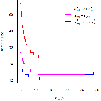
Fig. 3 Sample sizes under homo-
and heteroscedasticity (2×2×4 design).
Dashed lines at the switching
CV and the implied upper cap.
For our example we require 16 subjects under homoscedasticity (\(\small{CV_\textrm{wT}\equiv
CV_\textrm{wR}=12.5\%}\)) but 28 if \(\small{s_\textrm{wT}^2=2\times
s_\textrm{wR}^2}\). On the other hand, if \(\small{s_\textrm{wT}^2=0.5\times
s_\textrm{wR}^2}\), we require only twelve.
Starting with the implied upper cap at 21.4188% sample sizes
increase because the additional condition ‘must pass
ABE’ sets in.
Multiple Endpoints
In demonstrating bioequivalence the pharmacokinetic metrics Cmax, AUC0–t, and AUC0–∞ are mandatory.
We don’t have to worry about multiplicity issues (leading to an inflated Type I Error), since if all tests must pass at level \(\small{\alpha}\), we are protected by the intersection-union principle.23 24
We design the study always for the worst case combination, i.e., based on the PK metric requiring the largest sample size. Let’s explore that with different CVs and T/R-ratios.
metrics <- c("Cmax", "AUCt", "AUCinf")
CV      <- c(0.125, 0.100, 0.110)
theta0  <- c(0.975, 0.970, 0.980)
d.f     <- data.frame(metric = metrics, CV = CV, theta0 = theta0,
                      n = NA_integer_, power = NA_real_)
for (i in seq_along(metrics)) {
  d.f[i, 4:5] <- sampleN.NTID(CV = CV[i], theta0 = theta0[i],
                              details = FALSE, print = FALSE)[8:9]
}
d.f$power <- signif(d.f$power, 5)
txt       <- paste0("Sample size based on ",
                    d.f$metric[d.f$n == max(d.f$n)], ".\n")
print(d.f, row.names = FALSE)
cat(txt)
# metric CV theta0 n power
# Cmax 0.125 0.975 16 0.82278
# AUCt 0.100 0.970 18 0.80051
# AUCinf 0.110 0.980 16 0.83411
# Sample size based on AUCt.The PK metric with the lowest variability drives the sample size.
Let us assume for simplicity the same T/R-ratio of 0.975 for all metrics. Which are the extreme T/R-ratios (largest deviations of T from R) for Cmax giving still the target power?
opt <- function(x) {
  power.NTID(theta0 = x, CV = d.f$CV[1],
             n = d.f$n[2]) - target
}
metrics <- c("Cmax", "AUCt", "AUCinf")
CV      <- c(0.125, 0.100, 0.110)
theta0  <- 0.975
target  <- 0.80
d.f     <- data.frame(metric = metrics, CV = CV,
                      n = NA_integer_, power = NA_real_)
for (i in seq_along(metrics)) {
  d.f[i, 3:4] <- sampleN.NTID(CV = CV[i], theta0 = theta0,
                              details = FALSE, print = FALSE)[8:9]
}
d.f$power <- signif(d.f$power, 5)
if (theta0 < 1) {
  res <- uniroot(opt, tol = 1e-8,
                 interval = c(0.80 + 1e-4, theta0))
} else {
  res <- uniroot(opt, tol = 1e-8,
                 interval = c(theta0, 1.25 - 1e-4))
}
res     <- unlist(res)
theta0s <- c(res[["root"]], 1/res[["root"]])
txt     <- paste0("Target power for ", metrics[1],
                  " and sample size ",
                  d.f$n[2], "\nachieved for theta0 ",
                  sprintf("%.4f", theta0s[1]), " or ",
                  sprintf("%.4f", theta0s[2]), ".\n")
print(d.f, row.names = FALSE)
cat(txt)
# metric CV n power
# Cmax 0.125 16 0.82278
# AUCt 0.100 18 0.84179
# AUCinf 0.110 16 0.80470
# Target power for Cmax and sample size 18
# achieved for theta0 0.9626 or 1.0388.That means, although we assumed for Cmax the same T/R-ratio as for AUC, with the sample size of 18 required for AUCt, for Cmax it can be as low as ~0.963 or as high as ~1.039, which is an interesting side-effect.
Q & A
Q: Can we use
Rin a regulated environment and isPowerTOSTvalidated?
A: See this document25 about the acceptability of BaseRand its SDLC.26 It must be mentioned that the simulations which lead to the scaling-approach were performed by the FDA withRas well.27
Ris updated every couple of months with documented changes28 maintaining a bug-tracking system.29 I recommend to use always the latest release.
The authors ofPowerTOSTtried to do their best to provide reliable and valid results. The package’sNEWSdocuments the development of the package, bug-fixes, and introduction of new methods. Issues are tracked at GitHub (as of today none is still open). So far the package had >100,000 downloads. Therefore, it is extremely unlikely that bugs were not detected given its large user base.
The ultimate responsibility of validating any software (yes, of SAS as well…) lies in the hands of the user.30 31 32We can compare the – simulated – ABE-component of
power.NTID()with the exact power obtained bypower.TOST().
CV     <- sort(c(0.1002505, 0.214188, seq(0.11, 0.3, 0.01)))
theta0 <- 0.975
design <- "2x2x4"
res    <- data.frame(CV = CV, n = NA_integer_,
                     ABE.comp = NA_real_, exact = NA_real_,
                     RE = NA_character_)
for (i in seq_along(CV)) {
  res$n[i]        <- sampleN.NTID(CV  = CV[i],
                                  theta0 = theta0,
                                  design = design,
                                  print = FALSE,
                                  details = FALSE)[["Sample size"]]
  res$ABE.comp[i] <- suppressMessages(
                       power.NTID(CV  = CV[i],
                                  n = res$n[i],
                                  theta0 = theta0,
                                  design = design,
                                  details = TRUE)[["p(BE-ABE)"]])
  res$exact[i]    <- power.TOST(CV = CV[i],
                                n = res$n[i],
                                theta0 = theta0,
                                # use mixed-effects model's df
                                robust = TRUE,
                                design = design)
  res$RE[i] <- sprintf("%+.5f",
                       100 * (res$ABE.comp[i] - res$exact[i]) /
                       res$exact[i])
}
res$exact <- signif(res$exact, 5)
names(res)[5] <- "RE (%)"
print(res, row.names = FALSE)
# CV n ABE.comp exact RE (%)
# 0.1002505 18 1.00000 1.00000 +0.00000
# 0.1100000 16 1.00000 1.00000 +0.00001
# 0.1200000 16 1.00000 1.00000 +0.00019
# 0.1300000 16 0.99999 0.99998 +0.00069
# 0.1400000 16 0.99994 0.99991 +0.00330
# 0.1500000 16 0.99979 0.99964 +0.01484
# 0.1600000 16 0.99914 0.99894 +0.02021
# 0.1700000 16 0.99778 0.99742 +0.03604
# 0.1800000 16 0.99486 0.99462 +0.02402
# 0.1900000 16 0.99018 0.99004 +0.01402
# 0.2000000 16 0.98352 0.98321 +0.03109
# 0.2100000 16 0.97376 0.97376 +0.00040
# 0.2141880 16 0.96867 0.96894 -0.02828
# 0.2200000 16 0.96128 0.96140 -0.01200
# 0.2300000 16 0.94572 0.94599 -0.02813
# 0.2400000 16 0.92777 0.92751 +0.02851
# 0.2500000 16 0.90535 0.90604 -0.07634
# 0.2600000 16 0.88182 0.88177 +0.00519
# 0.2700000 18 0.90102 0.90075 +0.03008
# 0.2800000 18 0.87800 0.87768 +0.03630
# 0.2900000 18 0.85319 0.85245 +0.08653
# 0.3000000 20 0.87097 0.87168 -0.08166The maximum relative error is with +0.08653% negligible.
If you are not convinced, explore the relative error in repeated simulations with different seeds of the pseudo-random number generator.
CV.max <- res$CV[res[, 5] == max(res[, 5])]
n      <- sampleN.NTID(CV = CV.max, theta0 = theta0, design = design,
                          print = FALSE, details = FALSE)[["Sample size"]]
iter   <- 10L
runs   <- data.frame(run = 1:iter, seed = c(TRUE, rep(FALSE, iter - 1)),
                     ABE.comp = NA_real_, exact = NA_real_,
                     RE = NA_real_)
for (i in 1:iter) {
  set.seed(NULL)
  runs$ABE.comp[i] <- suppressMessages(
                        power.NTID(CV = CV.max, n = n, theta0 = theta0,
                                   design = design, details = TRUE,
                                   setseed = runs$seed[i])[["p(BE-ABE)"]])
  runs$exact[i]    <- power.TOST(CV = CV.max, n = n, theta0 = theta0,
                                 robust = TRUE, design = design)
  runs$RE[i]       <- 100 * (runs$ABE.comp[i] - runs$exact[i]) / runs$exact[i]
}
sum.RE         <- summary(runs$RE)
runs$exact     <- signif(runs$exact, 5)
runs$RE        <- sprintf("%+.5f", runs$RE)
names(runs)[5] <- "RE (%)"
print(runs, row.names = FALSE)
print(sum.RE)
# run seed ABE.comp exact RE (%)
# 1 TRUE 0.85319 0.85245 +0.08653
# 2 FALSE 0.85452 0.85245 +0.24255
# 3 FALSE 0.85366 0.85245 +0.14167
# 4 FALSE 0.85367 0.85245 +0.14284
# 5 FALSE 0.85099 0.85245 -0.17155
# 6 FALSE 0.85129 0.85245 -0.13635
# 7 FALSE 0.85156 0.85245 -0.10468
# 8 FALSE 0.85373 0.85245 +0.14988
# 9 FALSE 0.85425 0.85245 +0.21088
# 10 FALSE 0.85112 0.85245 -0.15630
# Min. 1st Qu. Median Mean 3rd Qu. Max.
# -0.17155 -0.12844 0.11410 0.04055 0.14812 0.24255Nothing to be worried about.
Q: I fail to understand your example about dropouts. We finish the study with 16 eligible subjects as desired. Why is the dropout-rate 20% and not the anticipated 15%?
A: That’s due to rounding up the calculated adjusted sample size (18.824…) to the next even number (20) in order to get balanced sequences.
If you manage it to dose fractional subjects (I can’t), the dropout rate would indeed equal the anticipated one because 100 × (1 – 16/18.824…) = 15%. ⬜Q: Do we have to worry about unbalanced sequences?
A:sampleN.NTID()will always give the total number of subjects for balanced sequences.
If you are interested in post hoc power, give the sample size as a vector, i.e.,power.NTID(..., n = c(foo, bar)), wherefooandbarare the number of subjects per sequence.Q: The default number of simulations in the sample size estimation is 100,000. Why?
A: We found that with this number the simulations are stable. Of course, you can give a larger number in the argumentnsims. However, you shouldn’t decrease the number.
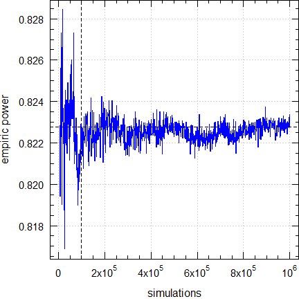
Fig. 4 Empiric power for
n = 16 (2×2×4 design).
Dashed lines give the result (0.8223)
obtained
by the default (100,00 simulations).
Q: How reliable are the results?
A: As stated in the Introduction, an exact method does not exist. We can only compare the empiric power of the ABE-component to the exact one obtained bypower.TOST(). For an example see above.Q: I still have questions. How to proceed?
A: The preferred method is to register at the BEBA Forum and post your question in the category or (please read the Forum’s Policy first).
You can contact me at [email protected]. Be warned – I will charge you for anything beyond most basic questions.
top of section ↩︎ previous section ↩︎
Licenses
 Helmut Schütz 2023
R and PowerTOST GPL 3.0,
klippy MIT,
pandoc GPL 2.0.
1st version January 01, 2022. Rendered June 21, 2023 10:52
CEST by rmarkdown via pandoc in 0.72 seconds.
Footnotes and References
Labes D, Schütz H, Lang B. PowerTOST: Power and Sample Size for (Bio)Equivalence Studies. Package version 1.5.4.9000. 2022-04-25. CRAN.↩︎
Labes D, Schütz H, Lang B. Package ‘PowerTOST’. February 21, 2022. CRAN.↩︎
FDA, OGD. Guidance on Warfarin Sodium. Rockville. Recommended Dec 2012. Download.↩︎
Endrényi L, Tóthfalusi L. Determination of Bioequivalence for Drugs with Narrow Therapeutic Index: Reduction of the Regulatory Burden. J Pharm Pharm Sci. 2013; 16(5): 676–82.
 Open
Access.↩︎
Open
Access.↩︎Yu LX, Jiang W, Zhang X, Lionberger R, Makhlouf F, Schuirmann DJ, Muldowney L, Chen ML, Davit B, Conner D, Woodcock J. Novel bioequivalence approach for narrow therapeutic index drugs. Clin Pharmacol Ther. 2015; 97(3): 286–91. doi:10.1002/cpt.28.↩︎
FDA, CDER. Draft Guidance for Industry. Bioequivalence Studies with Pharmacokinetic Endpoints for Drugs Submitted Under an ANDA. Rockville. August 2021. Download.↩︎
China Center for Drug Evaluation (CDE). Technical Guidance on Bioequivalence Studies of Drugs with Narrow Therapeutic Index. 2021.↩︎
Howe WG. Approximate Confidence Limits on the Mean of X+Y Where X and Y are Two Tabled Independent Random Variables. J Am Stat Assoc. 1974; 69(347): 789–94. doi:10.2307/2286019.↩︎
That’s contrary to methods for ABE, where the CV is an assumption as well.↩︎
Senn S. Guernsey McPearson’s Drug Development Dictionary. 21 April 2020. Online.↩︎
Hoenig JM, Heisey DM. The Abuse of Power: The Pervasive Fallacy of Power Calculations for Data Analysis. Am Stat. 2001; 55(1): 19–24. doi:10.1198/000313001300339897.
Open
Access.↩︎There is no statistical method to ‘correct’ for unequal carryover. It can only be avoided by design, i.e., a sufficiently long washout between periods. According to the guidelines subjects with pre-dose concentrations > 5% of their Cmax can by excluded from the comparison if stated in the protocol.↩︎
Senn S. Statistical Issues in Drug Development. New York: Wiley; 2nd ed 2007.↩︎
Note that you could specify other values for
alpha,theta1, ortheta2. However, this is not in accordance with the guidances and hence, not recommended.↩︎Zhang P. A Simple Formula for Sample Size Calculation in Equivalence Studies. J Biopharm Stat. 2003; 13(3): 529–38. doi:10.1081/BIP-120022772.↩︎
Generic NTIDs are expected by the FDA to meet assayed potency specifications of 95.0% to 105.0% instead of the common ±10%.↩︎
Yu LX. Quality and Bioequivalence Standards for Narrow Therapeutic Index Drugs. Presentation at: GPhA 2011 Fall Technical Workshop. Download.↩︎
Doyle AC. The Adventures of Sherlock Holmes. A Scandal in Bohemia. 1892. p 3.↩︎
Schütz H. Sample Size Estimation in Bioequivalence. Evaluation. 2020-10-23. BEBA Forum.↩︎
Lenth RV. Two Sample-Size Practices that I Don’t Recommend. October 24, 2000. Online.↩︎
The only exception is
design = "2x2x3"(the full replicate with three periods and sequences TRT|RTR). Then the first element is for sequence TRT and the second for RTR.↩︎Quoting my late father: »If you believe, go to church.«↩︎
Berger RL, Hsu JC. Bioequivalence Trials, Intersection-Union Tests and Equivalence Confidence Sets. Stat Sci. 1996; 11(4): 283–302. JSTOR:2246021.↩︎
Zeng A. The TOST confidence intervals and the coverage probabilities with R simulation. March 14, 2014. Online.↩︎
The R Foundation for Statistical Computing. A Guidance Document for the Use of R in Regulated Clinical Trial Environments. Vienna. October 18, 2021. Online.↩︎
The R Foundation for Statistical Computing. R: Software Development Life Cycle. A Description of R’s Development, Testing, Release and Maintenance Processes. Vienna. October 18, 2021. Online.↩︎
Jiang W, Makhlouf F, Schuirmann DJ, Zhang X, Zheng N, Conner D, Yu LX, Lionberger R. A Bioequivalence Approach for Generic Narrow Therapeutic Index Drugs: Evaluation of the Reference-Scaled Approach and Variability Comparison Criterion. AAPS J. 2015; 17(4) :891–901. doi:10.1208/s12248-015-9753-5.
 Free
Full Text.↩︎
Free
Full Text.↩︎ICH. Statistical Principles for Clinical Trials E9. 5 February 1998. Section 5.8. Online↩︎
FDA. Statistical Software Clarifying Statement. May 6, 2015. Download.↩︎
WHO. Guidance for organizations performing in vivo bioequivalence studies. Geneva. May 2016. Technical Report Series No. 996, Annex 9. Section 4.4. Online.↩︎