
Sample Size Estimation for Equivalence Studies in a Replicate Design
Helmut Schütz

July 24, 2024
Consider allowing JavaScript. Otherwise, you have to be proficient in
reading  since formulas
will not be rendered. Furthermore, the table of contents in the left
column for navigation will not be available and code-folding not
supported. Sorry for the inconvenience.
since formulas
will not be rendered. Furthermore, the table of contents in the left
column for navigation will not be available and code-folding not
supported. Sorry for the inconvenience.
Examples in this article were generated with
 4.4.1
by the package
4.4.1
by the package PowerTOST.1 More examples are
given in the respective vignette.2 See also the README on GitHub
for an overview and the Online manual3 for details.
- The right-hand badges give the respective section’s ‘level’.
- Basics about sample size methodology – requiring no or only limited statistical expertise.
- These sections are the most important ones. They are – hopefully – easily comprehensible even for novices.
- A somewhat higher knowledge of statistics and/or R is required. May be skipped or reserved for a later reading.
- An advanced knowledge of statistics and/or R is required. Not recommended for beginners in particular.
- If you are not a neRd or statistics afficionado, skipping is recommended. Suggested for experts but might be confusing for others.
- Click to show / hide R code.
- Click on the icon
 in the top left corner to copy R code to the
clipboard.
in the top left corner to copy R code to the
clipboard.
Abbreviations are given at the end.
Introduction
What are the main statistical issues in planning a confirmatory experiment?
For details about inferential statistics and hypotheses in equivalence see another article.
An ‘optimal’ study design is one, which – taking all assumptions into account – has a reasonably high chance of demonstrating equivalence (power) whilst controlling the patient’s risk.
Preliminaries
A basic knowledge of R is
required. To run the scripts at least version 1.4.3 (2016-11-01) of
PowerTOST is suggested. Any version of R would likely do, though the current release of
PowerTOST was only tested with R
4.3.3 (2024-02-29) and later. All scripts were run on a Xeon E3-1245v3 @
3.40GHz (1/4 cores) 16GB RAM with R 4.4.1 on
Windows 7 build 7601, Service Pack 1, Universal C Runtime
10.0.10240.16390.
Note that in all functions of PowerTOST the arguments
(say, the assumed T/R-ratio theta0, the
BE-limits (theta1,
theta2), the assumed coefficient of variation
CV, etc.) have to be given as ratios and not in
percent.
sampleN.TOST() gives balanced sequences (i.e.,
the same number of subjects is allocated to all sequences). Furthermore,
the estimated sample size is the total number of subjects (not
subjects per sequence – like in some other software packages).
Most examples deal with studies where the response variables likely
follow a log-normal
distribution, i.e., we assume a multiplicative model
(ratios instead of differences). We work with \(\small{\log_{e}}\)-transformed data in
order to allow analysis by the t-test (requiring differences).
This is the default in most functions of PowerTOST and
hence, the argument logscale = TRUE does not need to be
specified.
Terminology
It may sound picky but ‘sample size calculation’ (as used in most guidelines and alas, in some publications and textbooks) is sloppy terminology. In order to get prospective power (and hence, a sample size), we need five values:
- The level of the test \(\small{\alpha}\) (in BE commonly 0.05),
- the BE-margins (commonly 0.80 – 1.25),
- the desired (or target) power \(\small{\pi}\),
- the variance (commonly expressed as a coefficient of variation), and
- the deviation of the test from the reference treatment.
1 – 2 are fixed by the agency,
3 is set by the sponsor (commonly to 0.80 – 0.90), and
4 – 5 are just (uncertain!) assumptions.
In other words, obtaining a sample size is not an exact calculation like \(\small{2\times2=4}\) but always just an estimation.
“Power Calculation – A guess masquerading as mathematics.
Of note, it is extremely unlikely that all assumptions will be exactly realized in a particular study. Hence, calculating retrospective (a.k.a. post hoc, a posteriori) power is not only futile but plain nonsense.5
It is a prerequisite that no – unequal – carryover from one period to the next exists. Only then the comparison of treatments will be unbiased. For details see another article.6
Subjects have to be in the same physiological state7 throughout the study –
guaranteed by sufficiently long washout phases. Crossover studies can
not only be performed in healthy volunteers but also in patients with a
stable disease (e.g., asthma). Studies in patients
with an instable disease (e.g., in oncology)
must be performed in a parallel design (covered in another
article).
If crossovers are not feasible (e.g., for drugs with a very
long half life), studies could be performed in a parallel design as
well.
Power → Sample size
The sample size cannot be directly estimated, only
power –
exactly – calculated for an already given sample size.
The power equations cannot be re-arranged to solve for sample size. Instead, it is determined in an iterative procedure.
“Power. That which statisticians are always calculating but never have.

Contrary to parallel and 2×2×2 crossover designs I don’t give approximations for the sample size. Since there are numerous replicate designs possible (each with different degrees of freedom), the R code would be too long – even for my taste (Spaghetti viennese).
“Power: That which is wielded by the priesthood of clinical trials, the statisticians, and a stick which they use to beta their colleagues.
Let’s start with PowerTOST.
library(PowerTOST) # attach it to run the examplesIts sample size functions use a modification of Zhang’s method10 based
on the large sample approximation as the starting value of the
iterations You can unveil the course of iterations with
details = TRUE.
sampleN.TOST(CV = 0.45, theta0 = 0.95,
             targetpower = 0.80,
             design = "2x2x4", details = TRUE)
#
# +++++++++++ Equivalence test - TOST +++++++++++
# Sample size estimation
# -----------------------------------------------
# Study design: 2x2x4 (4 period full replicate)
# Design characteristics:
# df = 3*n-4, design const. = 1, step = 2
#
# log-transformed data (multiplicative model)
#
# alpha = 0.05, target power = 0.8
# BE margins = 0.8 ... 1.25
# True ratio = 0.95, CV = 0.45
#
# Sample size search (ntotal)
# n power
# 40 0.799409
# 42 0.818228
#
# Exact power calculation with
# Owen's Q functions.Two iterations. In many cases it hits the bull’s eye right away, i.e., already with the first guess.
We evaluate our studies based on the t-test, right?
The sample size based on the normal distribution may be too small, thus
compromising power.
#                     method  n Delta    RE    power
#       large sample approx. 40    -2 -4.8% 0.803974
#     central t-distribution 42    ±0 ±0.0% 0.817294
#  noncentral t-distribution 42    ±0 ±0.0% 0.818228
# exact method (Owen’s Q) 42 – – 0.818228Examples
Throughout the examples by I’m referring to studies in a single center – not multiple groups within them or multicenter studies. That’s another cup of tea. For some potential problems see another article.
A Simple Case
We assume a CV of 0.45, a T/R-ratio of 0.95, a target a power of 0.80, and want to perform the study in a four-period full replicate study with two sequences.
Since theta0 = 0.95, and targetpower = 0.80
are defaults of the function, we don’t have to give them explicitely. As
usual in bioequivalence, alpha = 0.05 is employed (we will
assess the study by a \(\small{100(1-2\,\alpha)=90\%}\) confidence
interval) and the BE-limits are
theta1 = 0.80 and theta2 = 1.25. Since they
are also defaults of the function, we don’t have to give them as well.
Hence, you need to specify only the CV and
design = "2x2x4".
sampleN.TOST(CV = 0.45, design = "2x2x4")#
# +++++++++++ Equivalence test - TOST +++++++++++
# Sample size estimation
# -----------------------------------------------
# Study design: 2x2x4 (4 period full replicate)
# log-transformed data (multiplicative model)
#
# alpha = 0.05, target power = 0.8
# BE margins = 0.8 ... 1.25
# True ratio = 0.95, CV = 0.45
#
# Sample size (total)
# n power
# 42 0.818228Sometimes we are not interested in the entire output and want to use
only a part of the results in subsequent calculations. We can suppress
the output by the argument print = FALSE and assign the
result to a data frame (here named x).
x <- sampleN.TOST(CV = 0.45, design = "2x2x4",
                  print = FALSE)
Although you could access the elements by the number of the column(s), I don’t recommend that, since in various functions these numbers are different and hence, difficult to remember.
Let’s retrieve the column names of x:
names(x)
# [1] "Design"         "alpha"          "CV"
# [4] "theta0"         "theta1"         "theta2"
# [7] "Sample size"    "Achieved power" "Target power"
Now we can access the elements of x by their names. Note
that double square brackets [[…]] have to be used.
x[["Sample size"]]
# [1] 42
x[["Achieved power"]]
# [1] 0.818228
Although you could access the elements by the number of the
column(s), I don’t recommend that, since in various other functions of
PowerTOST these numbers are different and hence, difficult
to remember. If you insist in accessing elements by column-numbers, use
single square brackets […].
x[7:8]
#   Sample size Achieved power
# 1          42       0.818228
With 42 subjects (21 per sequence) we achieve the power we desire.
What happens if we have one dropout?
power.TOST(CV = 0.45, design = "2x2x4",
           n = df[["Sample size"]] - 1)
# Unbalanced design. n(i)=21/20 assumed.# [1] 0.8088329Still above the 0.80 we desire. However, with two dropouts (40 eligible subjects) we would slightly fall short (0.7994).
Since dropouts are common, it makes sense to include / dose more subjects in order to end up with a number of eligible subjects which is not lower than our initial estimate.
Let us explore that in the next section.
Dropouts
We define two supportive functions:
- Provide equally sized sequences, i.e., any total sample
size
nwill be rounded up to achieve balance.
balance <- function(n, n.seq) {
  return(as.integer(n.seq * (n %/% n.seq + as.logical(n %% n.seq))))
}- Provide the adjusted sample size based on the original sample size
nand the anticipated droput-ratedo.rate.
nadj <- function(n, do.rate, n.seq) {
  return(as.integer(balance(n / (1 - do.rate), n.seq)))
}
In order to come up with a suggestion we have to anticipate a (realistic!) dropout rate. Note that this not the job of the statistician; ask the Principal Investigator.
“It is a capital mistake to theorize before one has data. Insensibly one begins to twist facts to suit theories, instead of theories to suit facts.
Dropout-rate
The dropout-rate is calculated from the eligible and
dosed subjects
or simply \[\begin{equation}\tag{3}
do.rate=1-n_\textrm{eligible}/n_\textrm{dosed}
\end{equation}\] Of course, we know it only after the
study was performed.
By substituting \(n_\textrm{eligible}\) with the estimated sample size \(n\), providing an anticipated dropout-rate and rearrangement to find the adjusted number of dosed subjects \(n_\textrm{adj}\) we should use \[\begin{equation}\tag{4} n_\textrm{adj}=\;\upharpoonleft n\,/\,(1-do.rate) \end{equation}\] where \(\upharpoonleft\) denotes rounding up to the next even number as implemented in the functions above.
An all too common mistake is to increase the estimated sample size \(n\) by the dropout-rate according to \[\begin{equation}\tag{5} n_\textrm{adj}=\;\upharpoonleft n\times(1+do.rate) \end{equation}\]
If you used \(\small{(5)}\) in the past – you are not alone. In a small survey a whopping 29% of respondents reported to use it.12 Consider changing your routine.
“There are no routine statistical questions, only questionable statistical routines.
Adjusted Sample Size
In the following I specified more arguments to make the function more
flexible.
Note that I wrapped the function power.TOST() in
suppressMessages(). Otherwise, the function will throw for
any odd sample size a message telling us that the design is
unbalanced. Well, we know that.
CV      <- 0.45 # within-subject CV
target  <- 0.80 # target (desired) power
theta0  <- 0.95 # assumed T/R-ratio
theta1  <- 0.80 # lower BE limit
theta2  <- 1.25 # upper BE limit
design  <- "2x2x4"
do.rate <- 0.10 # anticipated dropout-rate 10%
n.seq   <- as.integer(substr(design, 3, 3))
x       <- sampleN.TOST(CV = CV, theta0 = theta0,
                        theta1 = theta1,
                        theta2 = theta2,
                        targetpower = target,
                        design = design,
                        print = FALSE)
# calculate the adjusted sample size
n.adj   <- nadj(x[["Sample size"]], do.rate, n.seq)
# (decreasing) vector of eligible subjects
n.elig  <- n.adj:x[["Sample size"]]
info    <- paste0("Assumed CV              : ",
                  CV,
                  "\nAssumed T/R ratio       : ",
                  theta0,
                  "\nBE limits               : ",
                  paste(theta1, theta2, sep = "\u2026"),
                  "\nTarget (desired) power  : ",
                  target,
                  "\nAnticipated dropout-rate: ",
                  do.rate,
                  "\nEstimated sample size   : ",
                  x[["Sample size"]], " (",
                  x[["Sample size"]]/2, "/sequence)",
                  "\nAchieved power          : ",
                  signif(x[["Achieved power"]], 4),
                  "\nAdjusted sample size    : ",
                  n.adj, " (",  n.adj/2, "/sequence)",
                  "\n\n")
# explore the potential outcome for
# an increasing number of dropouts
do.act <- signif((n.adj - n.elig) / n.adj, 4)
x      <- data.frame(dosed    = n.adj,
                     eligible = n.elig,
                     dropouts = n.adj - n.elig,
                     do.act   = do.act,
                     power    = NA)
for (i in 1:nrow(df)) {
  x$power[i] <- suppressMessages(
                  power.TOST(CV = CV,
                             theta0 = theta0,
                             theta1 = theta1,
                             theta2 = theta2,
                             design = design,
                             n = x$eligible[i]))
}
cat(info)
print(round(x, 4), row.names = FALSE)
# Assumed CV : 0.45
# Assumed T/R ratio : 0.95
# BE limits : 0.8…1.25
# Target (desired) power : 0.8
# Anticipated dropout-rate: 0.1
# Estimated sample size : 42 (21/sequence)
# Achieved power : 0.8182
# Adjusted sample size : 48 (24/sequence)
#
# dosed eligible dropouts do.act power
# 48 48 0 0.0000 0.8645
# 48 47 1 0.0208 0.8576
# 48 46 2 0.0417 0.8506
# 48 45 3 0.0625 0.8429
# 48 44 4 0.0833 0.8352
# 48 43 5 0.1042 0.8267
# 48 42 6 0.1250 0.8182In the worst case (six dropouts) we end up with the originally estimated sample size of 42. Power preserved, mission accomplished. If we have less dropouts, splendid – we gain power.
If we would have adjusted the sample size acc. to \(\small{(5)}\) we
would have dosed also 48 subjects like the 48 acc. to \(\small{(4)}\).
Cave: This might not always be the case… If the anticipated dropout rate
of 10% is realized in the study, we would have also 43 eligible subjects
(power 0.8267). In this example we achieve still more than our target
power but the loss might be relevant in other cases.
Post hoc Power
As said in the preliminaries, calculating post hoc power is futile.
“There is simple intuition behind results like these: If my car made it to the top of the hill, then it is powerful enough to climb that hill; if it didn’t, then it obviously isn’t powerful enough. Retrospective power is an obvious answer to a rather uninteresting question. A more meaningful question is to ask whether the car is powerful enough to climb a particular hill never climbed before; or whether a different car can climb that new hill. Such questions are prospective, not retrospective.
However, sometimes we are interested in it for planning the next study.
If you give and odd total sample size n,
power.TOST() will try to keep sequences as balanced as
possible and show in a message how that was done.
n.act <- 41
signif(power.TOST(CV = 0.45, n = n.act, design = "2x2x4"), 6)
# Unbalanced design. n(i)=21/20 assumed.# [1] 0.808833Say, our study was more unbalanced. Let us assume that we dosed 48
subjects, the total number of subjects was also 41 but all dropouts
occured in one sequence (unlikely but possible).
Instead of the total sample size n we can give the number
of subjects of each sequence as a vector (the order is not relevant,
i.e., it does not matter which element refers to the
TRTR or RTRT sequence).
n.adj    <- 48
n.act    <- 41
n.s1     <- n.adj / 2
n.s2     <- n.act - n.s1
post.hoc <- signif(power.TOST(CV  = 0.45,
                             n = c(n.s1, n.s2),
                             design = "2x2x4"), 6)
sig.dig  <- nchar(as.character(n.adj))
fmt      <- paste0("%", sig.dig, ".0f (%",  sig.dig, ".0f dropouts)")
cat(paste0("Dosed subjects: ", sprintf("%2.0f", n.adj),
           "\nEligible      : ",
           sprintf(fmt, n.act, n.adj - n.act),
           "\n  Sequence 1  : ",
           sprintf(fmt, n.s1, n.adj / 2 - n.s1),
           "\n  Sequence 1  : ",
           sprintf(fmt, n.s2, n.adj / 2 - n.s2),
           "\nPower         :  ", post.hoc, "\n"))
# Dosed subjects: 48
# Eligible : 41 ( 7 dropouts)
# Sequence 1 : 24 ( 0 dropouts)
# Sequence 1 : 17 ( 7 dropouts)
# Power : 0.797608Of course, in a particular study you will provide the numbers in the
n vector directly.
Lost in Assumptions
As stated already in the Introduction, the
CV and the T/R-ratio are only assumptions. Whatever
their origin might be (literature, previous studies) they carry some
degree of uncertainty. Hence, believing14 that they are the
true ones may be risky.
Some statisticians call that the ‘Carved-in-Stone’ approach.
Say, we performed a pilot study in 16 subjects and estimated the CV as 0.45.
The \(\alpha\) confidence interval of the CV is obtained via the \(\small{\chi^2}\)-distribution of its error variance \(\small{\sigma^2}\) with \(\small{n-2}\) degrees of freedom. \[\eqalign{\tag{6} s_\text{w}^2&=\log_{e}(CV_\text{w}^2+1)\\ L=\frac{(n-1)\,s_\text{w}^2}{\chi_{\alpha/2,\,n-2}^{2}}&\leq\sigma_\text{w}^2\leq\frac{(n-1)\,s_\text{w}^2}{\chi_{1-\alpha/2,\,n-2}^{2}}=U\\ \left\{lower\;CL,\;upper\;CL\right\}&=\left\{\sqrt{\exp(L)-1},\sqrt{\exp(U)-1}\right\} }\]
Let’s calculate the 95% confidence interval of the CV to get an idea.
m  <- 16 # pilot study
ci <- CVCL(CV = 0.45, df = m - 2,
           side = "2-sided", alpha = 0.05)
signif(ci, 4)
# lower CL upper CL
# 0.3223 0.7629Surprised? Although 0.45 is the best estimate for planning the next study, there is no guarantee that we will get exactly the same outcome. Since the \(\small{\chi^2}\)-distribution is skewed to the right, it is more likely to face a higher CV than a lower one in the pivotal study.
If we plan the study based on 0.45, we would opt for 42 subjects like
in the examples before (not adjusted for the dropout-rate).
If the CV will be lower, we gain power. Fine.
But what if it will be higher? Of course, we will loose power. But how
much?
Let’s explore what might happen at the confidence limits of the CV.
m    <- 16
ci   <- CVCL(CV = 0.45, df = m - 2,
             side = "2-sided", alpha = 0.05)
n    <- 28
comp <- data.frame(CV = c(ci[["lower CL"]], 0.45,
                          ci[["upper CL"]]),
                   power = NA)
for (i in 1:nrow(comp)) {
  comp$power[i] <- power.TOST(CV = comp$CV[i],
                              n = n)
}
comp[, 1] <- signif(comp[, 1], 4)
comp[, 2] <- signif(comp[, 2], 6)
print(comp, row.names = FALSE)
# CV power
# 0.3223 0.57315300
# 0.4500 0.19171300
# 0.7629 0.00127429Ouch!
What can we do? The larger the previous study was, the larger the degrees of freedom and hence, the narrower the confidence interval of the CV. In simple terms: The estimate is more certain. On the other hand, it also means that very small pilot studies are practically useless.
m               <- seq(12, 24, 6)
x               <- data.frame(n = m, CV = 0.45,
                              l = NA, u = NA)
for (i in 1:nrow(x)) {
  x[i, 3:4] <- CVCL(CV = 0.45, df = m[i] - 2,
                    side = "2-sided",
                    alpha = 0.05)
}
x[, 3:4]      <- signif(x[, 3:4], 4)
names(x)[3:4] <- c("lower CL", "upper CL")
print(x, row.names = FALSE)
# n CV lower CL upper CL
# 12 0.45 0.3069 0.8744
# 18 0.45 0.3282 0.7300
# 24 0.45 0.3415 0.6685A Bayesian
method is implemented in PowerTOST, which takes
the uncertainty of estimates into account. We can explore the
uncertainty of the CV or the T/R-ratio and of both.
m      <- 16   # sample size of pilot
CV     <- 0.45
theta0 <- 0.95
x      <- expsampleN.TOST(CV = CV, theta0 = theta0,
                          targetpower = 0.80,
                          design = "2x2x4",
                          prior.parm = list(
                            m = m, design = "2x2x4"),
                          prior.type = "CV", # uncertain CV
                          details = FALSE)
#
# ++++++++++++ Equivalence test - TOST ++++++++++++
# Sample size est. with uncertain CV
# -------------------------------------------------
# Study design: 2x2x4 replicate crossover
# log-transformed data (multiplicative model)
#
# alpha = 0.05, target power = 0.8
# BE margins = 0.8 ... 1.25
# Ratio = 0.95
# CV = 0.45 with 44 df
#
# Sample size (ntotal)
# n exp. power
# 42 0.800179Good that our pilot was in a fully replicated design (large degrees of freedom).
What about an uncertain T/R-ratio?
m      <- 16
CV     <- 0.45
theta0 <- 0.95
x      <- expsampleN.TOST(CV = CV, theta0 = theta0,
                          targetpower = 0.80,
                          design = "2x2x4",
                          prior.parm = list(
                            m = m, design = "2x2x4"),
                          prior.type = "theta0", # uncertain T/R-ratio
                          details = FALSE)
#
# ++++++++++++ Equivalence test - TOST ++++++++++++
# Sample size est. with uncertain theta0
# -------------------------------------------------
# Study design: 2x2x4 replicate crossover
# log-transformed data (multiplicative model)
#
# alpha = 0.05, target power = 0.8
# BE margins = 0.8 ... 1.25
# Ratio = 0.95
# CV = 0.45
#
# Sample size (ntotal)
# n exp. power
# 128 0.800005Terrible! The sample size more than doubles.
That should not take us by surprise. We don’t know where the true T/R-ratio lies but we can calculate the lower 95% confidence limit of the pilot study’s point estimate to get an idea about a worst case.
m      <- 16
CV     <- 0.45
pe     <- 0.95
ci     <- round(CI.BE(CV = CV, pe = 0.95, n = m,
                      design = "2x2x4"), 4)
if (pe <= 1) {
  cl <- ci[["lower"]]
} else {
  cl <- ci[["upper"]]
}
print(cl)
# [1] 0.7932Explore the impact of a relatively 5% higher CV and a relatively 5% lower T/R-ratio on power for a given sample size.
n      <- 42
CV     <- 0.45
theta0 <- 0.95
comp1  <- data.frame(CV = c(CV, CV*1.05),
                     power = NA)
comp2  <- data.frame(theta0 = c(theta0, theta0*0.95),
                     power = NA)
for (i in 1:2) {
  comp1$power[i] <- power.TOST(CV = comp1$CV[i],
                               theta0 = theta0,
                               design = "2x2x4",
                               n = n)
}
comp1$power <- signif(comp1$power, 6)
for (i in 1:2) {
  comp2$power[i] <- power.TOST(CV = CV,
                               theta0 = comp2$theta0[i],
                               design = "2x2x4",
                               n = n)
}
comp2$power <- signif(comp2$power, 6)
print(comp1, row.names = FALSE)
print(comp2, row.names = FALSE)
# CV power
# 0.4500 0.818228
# 0.4725 0.783684
# theta0 power
# 0.9500 0.818228
# 0.9025 0.564727Interlude 1
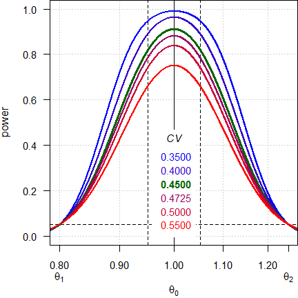
Fig. 1 Power curves for n = 42, 2×2×4 design.
Note the log-scale of the x-axis. It demonstrates that power curves are symmetrical around 1 (\(\small{\log_{e}(1)=0}\), where \(\small{\log_{e}(\theta_2)=\left|\log_{e}(\theta_1)\right|}\)) and we will achieve the same power for \(\small{\theta_0}\) and \(\small{1/\theta_0}\) (e.g., for 0.95 and 1.0526). Furthermore, all curves intersect 0.05 at \(\small{\theta_1}\) and \(\small{\theta_2}\), which means that for a true \(\small{\theta_0}\) at one of the limits \(\small{\alpha}\) is strictly controlled.
<nitpick>-
A common flaw in protocols is the phrase
»The sample size was calculated [sic] based on a T/R-ratio of 0.95 – 1.05…«
If you assume a deviation of 5% of the test from the reference and are not sure about its direction (lower or higer than 1), always use the lower T/R-ratio. If you would use the upper T/R-ratio, power would be only preserved down to 1/1.05 = 0.9524.
Given, sometimes you will need a higher sample size with the lower T/R-ratio. There’s no free lunch.
CV      <- 0.45
delta   <- 0.05 # direction unknown
design  <- "2x2x4"
theta0s <- c(1 - delta, 1 / (1 + delta),
             1 + delta, 1 / (1 - delta))
n       <- sampleN.TOST(CV = CV, theta0 = 1 - delta,
                        design = design,
                        print = FALSE)[["Sample size"]]
comp1   <- data.frame(CV = CV, theta0 = theta0s,
                      base = c(TRUE, rep(FALSE, 3)),
                      n = n, power = NA)
for (i in 1:nrow(comp1)) {
  comp1$power[i] <- power.TOST(CV = CV,
                               theta0 = comp1$theta0[i],
                               design = design, n = n)
}
n       <- sampleN.TOST(CV = CV, theta0 = 1 + delta,
                        design = design,
                        print = FALSE)[["Sample size"]]
comp2   <- data.frame(CV = CV, theta0 = theta0s,
                      base = c(FALSE, FALSE, TRUE, FALSE),
                      n = n, power = NA)
for (i in 1:nrow(comp2)) {
  comp2$power[i] <- power.TOST(CV = CV,
                               theta0 = comp2$theta0[i],
                               design = design, n = n)
}
comp1[, c(2, 5)] <- signif(comp1[, c(2, 5)] , 4)
comp2[, c(2, 5)] <- signif(comp2[, c(2, 5)] , 4)
print(comp1, row.names = FALSE)
print(comp2, row.names = FALSE)
# CV theta0 base n power
# 0.45 0.9500 TRUE 42 0.8182
# 0.45 0.9524 FALSE 42 0.8270
# 0.45 1.0500 FALSE 42 0.8270
# 0.45 1.0530 FALSE 42 0.8182
# CV theta0 base n power
# 0.45 0.9500 FALSE 40 0.7994
# 0.45 0.9524 FALSE 40 0.8083
# 0.45 1.0500 TRUE 40 0.8083
# 0.45 1.0530 FALSE 40 0.7994Since power is much more sensitive to the T/R-ratio than to the CV, the results obtained with the Bayesian method should be clear now.
Essentially this leads to the murky waters of prospective power and sensitivity analyses,
which are covered in other articles.
An appetizer to show the maximum deviations (CV, T/R-ratio and
decreased sample size due to dropouts) which give still a minimum
acceptable power of ≥ 0.70:
CV       <- 0.45
theta0   <- 0.95
target   <- 0.80
minpower <- 0.70
pa       <- pa.ABE(CV = CV, theta0 = theta0,
                   targetpower = target,
                   minpower = minpower,
                   design = "2x2x4")
change.CV     <- 100*(tail(pa$paCV[["CV"]], 1) -
                      pa$plan$CV) / pa$plan$CV
change.theta0 <- 100*(head(pa$paGMR$theta0, 1) -
                      pa$plan$theta0) /
                      pa$plan$theta0
change.n      <- 100*(tail(pa$paN[["N"]], 1) -
                      pa$plan[["Sample size"]]) /
                      pa$plan[["Sample size"]]
comp     <- data.frame(parameter = c("CV", "theta0", "n"),
                       change = c(change.CV,
                                  change.theta0,
                                  change.n))
comp$change <- sprintf("%+.2f%%", comp$change)
names(comp)[2] <- "relative change"
print(pa, plotit = FALSE)
print(comp, row.names = FALSE)
# Sample size plan ABE
# Design alpha CV theta0 theta1 theta2 Sample size
# 2x2x4 0.05 0.45 0.95 0.8 1.25 42
# Achieved power
# 0.818228
#
# Power analysis
# CV, theta0 and number of subjects leading to min. acceptable power of ~0.7:
# CV= 0.5247, theta0= 0.9248
# n = 32 (power= 0.7005)
#
# parameter relative change
# CV +16.60%
# theta0 -2.66%
# n -23.81%Confirms what we have seen above. Interesting that the sample size is the least sensitive one. Many overrate the impact of dropouts on power.
If you didn’t stop reading in desperation (understandable), explore both uncertain CV and T/R-ratio:
m      <- 16
CV     <- 0.45
theta0 <- 0.95
x      <- expsampleN.TOST(CV = CV, theta0 = theta0,
                          targetpower = 0.80,
                          design = "2x2x4",
                          prior.parm = list(
                            m = m, design = "2x2x4"),
                          prior.type = "both", # uncertain CV and T/R-ratio
                          details = FALSE)
#
# ++++++++++++ Equivalence test - TOST ++++++++++++
# Sample size est. with uncertain CV and theta0
# -------------------------------------------------
# Study design: 2x2x4 replicate crossover
# log-transformed data (multiplicative model)
#
# alpha = 0.05, target power = 0.8
# BE margins = 0.8 ... 1.25
# Ratio = 0.95 with 44 df
# CV = 0.45 with 44 df
#
# Sample size (ntotal)
# n exp. power
# 142 0.800556I don’t suggest that you should use it in practice. AFAIK, not even the main author of this function (Benjamin Lang) does. However, it serves educational purposes to show that it is not that easy and why even properly planned studies might fail.
An alternative to assuming a T/R-ratio is based on statistical
assurance.15 This concept uses the distribution of
T/R-ratios and assumes an uncertainty parameter \(\small{\sigma_\textrm{u}}\). A natural
assumption is \(\small{\sigma_\textrm{u}=1-\theta_0}\),
i.e., for the commonly applied T/R-ratio of 0.95 one can use
the argument sem = 0.05 in the function
expsampleN.TOST(), where the argument theta0
has to be fixed at 1.
CV        <- 0.45
theta0    <- 0.95
target    <- 0.80
sigma.u   <- 1 - theta0
comp      <- data.frame(theta0 = theta0,
                        n.1 = NA, power = NA,
                        sigma.u = sigma.u,
                        n.2 = NA, assurance = NA)
comp[2:3] <- sampleN.TOST(CV = CV,
                          targetpower = target,
                          theta0 = theta0,
                          design = "2x2x4",
                          details = FALSE,
                          print = FALSE)[7:8]
comp[5:6] <- expsampleN.TOST(CV = CV,
                             theta0 = 1, # fixed!
                             targetpower = target,
                             design = "2x2x4",
                             prior.type = "theta0",
                             prior.parm =
                               list(sem = sigma.u),
                             details = FALSE,
                             print = FALSE)[9:10]
names(comp)[c(2, 5)]  <- rep("n", 2)
print(signif(comp, 6), row.names = FALSE)
# theta0 n power sigma.u n assurance
# 0.95 42 0.818228 0.05 40 0.80949Multiple Endpoints
It is common that equivalence of more than one endpoint has to be demonstrated. In bioequivalence the pharmacokinetic metrics Cmax and AUC0–t are mandatory (in some jurisdictions like the FDA additionally AUC0–∞).
We don’t have to worry about multiplicity issues (inflated Type I Error), since if all tests must pass at level \(\small{\alpha}\), we are protected by the intersection-union principle.16 17
We design the study always for the worst case combination, i.e., based on the PK metric requiring the largest sample size. In some jurisdictions wider BE limits for Cmax are acceptable. Let’s explore that with different CVs and T/R-ratios.
metrics <- c("Cmax", "AUCt", "AUCinf")
CV      <- c(0.45, 0.35, 0.37)
theta0  <- c(0.95, 1.04, 1.06)
theta1  <- c(0.75, 0.80, 0.80)
theta2  <- 1 / theta1
target  <- 0.80
x       <- data.frame(metric = metrics,
                      theta1 = theta1, theta2 = theta2,
                      CV = CV, theta0 = theta0, n = NA)
for (i in 1:nrow(x)) {
  x$n[i] <- sampleN.TOST(CV = CV[i],
                         theta0 = theta0[i],
                         theta1 = theta1[i],
                         theta2 = theta2[i],
                         targetpower = target,
                         design = "2x2x4",
                         print = FALSE)[["Sample size"]]
}
x$theta1 <- sprintf("%.4f", x$theta1)
x$theta2 <- sprintf("%.4f", x$theta2)
txt       <- paste0("Sample size driven by ",
                    x$metric[x$n == max(x$n)], ".\n")
print(x, row.names = FALSE); cat(txt)
# metric theta1 theta2 CV theta0 n
# Cmax 0.7500 1.3333 0.45 0.95 24
# AUCt 0.8000 1.2500 0.35 1.04 24
# AUCinf 0.8000 1.2500 0.37 1.06 32
# Sample size driven by AUCinf.Even if we assume the same T/R-ratio for two PK metrics, we will get a wider margin for the one with lower variability.
Let’s continue with the conditions of our previous examples, this time assuming that the CV and T/R-ratio were applicable for Cmax. As common in PK, the CV of AUC is lower, say only 0.20. That means, the study is ‘overpowered’ for the assumed T/R-ratio of AUC.
Which are the extreme T/R-ratios (largest deviations of T from R) giving still the target power?
opt <- function(y) {
  power.TOST(theta0 = y, CV = x$CV[2],
             theta1 = theta1,
             theta2 = theta2,
             design = design,
             n = x$n[1]) - target
}
metrics <- c("Cmax", "AUC")
CV      <- c(0.45, 0.30) # Cmax, AUC
theta0  <- 0.95          # both metrics
theta1  <- 0.80
theta2  <- 1.25
target  <- 0.80
design  <- "2x2x4"
x       <- data.frame(metric = metrics, theta0 = theta0,
                      CV = CV, n = NA, power = NA)
for (i in 1:nrow(x)) {
  x[i, 4:5] <- sampleN.TOST(CV = CV[i],
                            theta0 = theta0,
                            theta1 = theta1,
                            theta2 = theta2,
                            targetpower = target,
                            design = design,
                            print = FALSE)[7:8]
}
x$power <- signif(x$power, 6)
if (theta0 < 1) {
  res <- uniroot(opt, tol = 1e-8,
                 interval = c(theta1 + 1e-4, theta0))
} else {
  res <- uniroot(opt, tol = 1e-8,
                 interval = c(theta0, theta2 - 1e-4))
}
res     <- unlist(res)
theta0s <- c(res[["root"]], 1/res[["root"]])
txt     <- paste0("Target power for ", metrics[2],
                 " and sample size ",
                 x$n[1], "\nachieved for theta0 ",
                 sprintf("%.4f", theta0s[1]), " or ",
                 sprintf("%.4f", theta0s[2]), ".\n")
print(x, row.names = FALSE)
cat(txt)
# metric theta0 CV n power
# Cmax 0.95 0.45 42 0.818228
# AUC 0.95 0.30 20 0.820240
# Target power for AUC and sample size 42
# achieved for theta0 0.8959 or 1.1161.That means, although we assumed for AUC the same T/R-ratio as for Cmax – with the sample size of 42 required for Cmax – for AUC it can be as low as ~0.90 or as high as ~1.12, which is a soothing side-effect.
Furthermore, sometimes we have less data of AUC than of Cmax (samples at the end of the profile missing or unreliable \(\small{\widehat{\lambda}_\textrm{z}}\) in some subjects and therefore, less data of AUC0–∞ than of AUC0–t). Again, it will not hurt because for the originally assumed T/R-ratio we need only 20 subjects.
Since – as a one-point metric – Cmax is
inherently more variable than AUC, Health Canada does not
require assessment of a confidence interval. Only the T/R-ratio has to
lie within 80.0 – 125.0%. We can explore that by setting
alpha = 0.5 for it.18
metrics <- c("Cmax", "AUC")
CV      <- c(0.90, 0.30)
theta0  <- 0.95
target  <- 0.80
design  <- "2x2x4"
alpha   <- c(0.50, 0.05)
x       <- data.frame(metric = metrics, CV = CV, theta0 = theta0,
                      alpha = alpha, n = NA)
for (i in 1:nrow(x)) {
  x$n[i] <- sampleN.TOST(alpha = alpha[i],
                         CV = CV[i],
                         theta0 = theta0,
                         targetpower = target,
                         design = design,
                         print = FALSE)[["Sample size"]]
}
txt       <- paste0("Sample size driven by ",
                     x$metric[x$n == max(x$n)], ".\n")
print(x, row.names = FALSE); cat(txt)
# metric CV theta0 alpha n
# Cmax 0.9 0.95 0.50 22
# AUC 0.3 0.95 0.05 20
# Sample size driven by Cmax.Only if the CV of Cmax is substantially higher than the one of AUC, you may face a situation where you have to base the sample size on Cmax.
NTIDs
So far we employed the common (and hence, default)
BE-limits theta1 = 0.80
and theta2 = 1.25. In some jurisdictions tighter limits of
90.00 – 111.11% have to be used.19
Generally NTIDs show a low within-subject variability (though the between-subject CV can be much higher – these drugs require quite often dose-titration).
You have to provide only the lower
BE-limit theta1 (the
upper one will be automatically calculated). In the examples I used a
lower CV of 0.125.
sampleN.TOST(CV = 0.125, theta1 = 0.90, design = "2x2x4")#
# +++++++++++ Equivalence test - TOST +++++++++++
# Sample size estimation
# -----------------------------------------------
# Study design: 2x2x4 (4 period full replicate)
# log-transformed data (multiplicative model)
#
# alpha = 0.05, target power = 0.8
# BE margins = 0.9 ... 1.111111
# True ratio = 0.95, CV = 0.125
#
# Sample size (total)
# n power
# 34 0.807718Doable.
Interlude 2
Health Canada requires for NTIDs (termed by HC ‘critical dose drugs’) that the confidence interval of Cmax lies within 80.0 – 125.0% and the one of AUC within 90.0 – 112.0%.
<nitpick>»These numbers are more easy to remember.«
</nitpick>
Hence, for Health Canada you have to set both limits.
sampleN.TOST(CV = 0.125, theta1 = 0.90, theta2 = 1.12,
             design = "2x2x4")
#
# +++++++++++ Equivalence test - TOST +++++++++++
# Sample size estimation
# -----------------------------------------------
# Study design: 2x2x4 (4 period full replicate)
# log-transformed data (multiplicative model)
#
# alpha = 0.05, target power = 0.8
# BE margins = 0.9 ... 1.12
# True ratio = 0.95, CV = 0.125
#
# Sample size (total)
# n power
# 34 0.807718Here we require the same sample size than with the common limits for NTIDs.
If you expect a T/R-ratio closer to 1, possibly you require two subjects less:
target  <- 0.80
theta0  <- 0.975
CV.min  <- 0.075
CV.max  <- 0.20
CV.step <- 1000
CV      <- seq(CV.min, CV.max, length.out = CV.step)
res     <- data.frame(CV = CV, n.EMA = NA_integer_,
                      n.HC = NA_integer_, less = FALSE)
for (i in 1:nrow(res)) {
  res$n.EMA[i] <- sampleN.TOST(CV = CV[i], theta0 = theta0,
                        targetpower = target, design = "2x2x4",
                        theta1 = 0.90, theta2 = 1/0.90,
                        print = FALSE)[["Sample size"]]
  res$n.HC[i]  <- sampleN.TOST(CV = CV[i], theta0 = theta0,
                        targetpower = target, design = "2x2x4",
                        theta1 = 0.90, theta2 = 1.12,
                        print = FALSE)[["Sample size"]]
  if (res$n.HC[i] < res$n.EMA[i]) res$less[i] = TRUE
}
cat("target power                :", target,
    "\ntheta0                      :", theta0,
    "\nCV                          :", CV.min, "\u2013", CV.max,
    "\nSample size for HC < common :",
    sprintf("%.2f%%", 100 * sum(res$less) / CV.step),
    "of cases.\n")
# target power : 0.8
# theta0 : 0.975
# CV : 0.075 – 0.2
# Sample size for HC < common : 9.40% of cases.The FDA requires for NTIDs tighter batch-release specifications (±5% instead of ±10%). Let’s hope that your product complies and the T/R-ratio will be closer to 1:
sampleN.TOST(CV = 0.125,
             theta0 = 0.975, # ‘better’ T/R-ratio
             theta1 = 0.90,
             design = "2x2x4")
#
# +++++++++++ Equivalence test - TOST +++++++++++
# Sample size estimation
# -----------------------------------------------
# Study design: 2x2x4 (4 period full replicate)
# log-transformed data (multiplicative model)
#
# alpha = 0.05, target power = 0.8
# BE margins = 0.9 ... 1.111111
# True ratio = 0.975, CV = 0.125
#
# Sample size (total)
# n power
# 16 0.805921Substantially lower sample size. That’s nice.
Difference of Means
Sometimes we are interested in assessing differences of responses and
not their ratios. In such a case we have to set
logscale = FALSE. The limits theta1 and
theta2 can be expressed in the following ways:
- As a difference of means relative to the same (underlying) reference mean.
- In units of the difference of means.
Note that in the former case the units of CV, and
theta0 need also to be given relative to the reference mean
(specified as a ratio).
Let’s estimate the sample size for an equivalence trial of two blood pressure lowering drugs assessing the difference in means of untransformed data (raw, linear scale). In this setup everything has to be given with the same units (i.e., here the assumed difference –5 mm Hg and the lower / upper limits ∓15 mm Hg systolic blood pressure). Furthermore, we assume a CV of 25 mm Hg.
sampleN.TOST(CV = 20, theta0 = -5,
             theta1 = -15, theta2 = +15,
             logscale = FALSE,
             design = "2x2x4")
#
# +++++++++++ Equivalence test - TOST +++++++++++
# Sample size estimation
# -----------------------------------------------
# Study design: 2x2x4 (4 period full replicate)
# untransformed data (additive model)
#
# alpha = 0.05, target power = 0.8
# BE margins = -15 ... 15
# True diff. = -5, CV = 20
#
# Sample size (total)
# n power
# 26 0.810576Sometimes in the literature we find not the CV but the standard deviation of the difference. Say, it is given with 36 mm Hg. We have to convert it to a CV.
SD.delta <- 36
design   <- "2x2x4"
# extract relevant information and retrieve design constant
known    <- known.designs()[7:11, c(2, 6, 9)]
bk       <- known[known$design == design, "bk"] #
sampleN.TOST(CV = SD.delta / sqrt(bk), theta0 = -5,
             theta1 = -15, theta2 = +15,
             logscale = FALSE,
             design = "2x2x4")
#
# +++++++++++ Equivalence test - TOST +++++++++++
# Sample size estimation
# -----------------------------------------------
# Study design: 2x2x4 (4 period full replicate)
# untransformed data (additive model)
#
# alpha = 0.05, target power = 0.8
# BE margins = -15 ... 15
# True diff. = -5, CV = 36
#
# Sample size (total)
# n power
# 82 0.805692For the 2×2×4 design the CV equals the SD because
the design constant bk is 1. However, that’s not true for
all replicate design. Show them:
#  design  bk                      name
#   2x2x3 1.5 2x2x3 replicate crossover
#   2x2x4 1.0 2x2x4 replicate crossover
#   2x4x4 1.0 2x4x4 replicate crossover
#   2x3x3 1.5 partial replicate (2x3x3)
#   2x4x2 8.0          Balaam's (2x4x2)
Note that other software packages (e.g., PASS, nQuery, StudySize, …) require the standard deviation of the difference as input.
Methods
“He who seeks for methods without having a definite problem in mind seeks in the most part in vain.
With a few exceptions (i.e., simulation-based methods), in
PowerTOST the default method = "exact"
implements Owen’s Q function20 which is also used in SAS’
Proc Power.
Other implemented methods are "mvt" (based on the
bivariate noncentral t-distribution),
"noncentral" / "nct" (noncentral
t-distribution), and "shifted" /
"central" (shifted central t-distribution).
Although "mvt" is also exact, it may have a somewhat lower
precision compared to Owen’s Q and has a much longer run-time.
Let’s compare them.
methods <- c("exact", "mvt", "noncentral", "central")
x       <- data.frame(method = methods,
                      power = rep(NA, 4))
for (i in 1:nrow(x)) {
  x$power[i] <- power.TOST(CV     = 0.45,
                           n      = 42,
                           design = "2x2x4",
                           method = x$method[i])
}
x$power <- round(x$power, 5)
print(x, row.names = FALSE)
# method power
# exact 0.81823
# mvt 0.81823
# noncentral 0.81823
# central 0.81729Power approximated by the shifted central t-distribution is
generally slightly lower compared to the others. Hence, if used in
sample size estimations, occasionally two more subjects are
‘required’.
Therefore, I recommend to use "method = shifted" /
"method = central" only for comparing with old results
(literature, own studies).
Q & A
Q: Can we use R in a regulated environment and is
PowerTOSTvalidated?
A: See this document21 about the acceptability of BaseRand its SDLC.22 It must be mentioned that the simulations which lead to the scaling-approach for NTIDs were performed by the FDA withR.23
Ris updated every couple of months with documented changes24 and maintaining a bug-tracking system.25 I recommend to use always the latest release.
The authors ofPowerTOSTtried to do their best to provide reliable and valid results. The package’sNEWSdocuments the development of the package, bug-fixes, and introduction of new methods. Issues are tracked at GitHub (as of today none is still open). So far the package had >118,000 downloads. Therefore, it is extremely unlikely that bugs were not detected given its large user base.
The ultimate responsibility of validating any software (yes, of SAS as well…) lies in the hands of the user.26 27 28Q: Which of the methods should we use in our daily practice?
A:method = exact. Full stop. Why rely on approximations? Since it is the default insampleN.TOST()andpower.TOST(), you don’t have to give this argument (saves keystrokes).Q: I fail to understand your example about dropouts. We finish the study with 42 eligible subjects as desired. Why is the dropout-rate ~12% and not the anticipated 10%?
A: That’s due to rounding up the calculated adjusted sample size (46.67…) to the next even number (48) in order to get balanced sequences. If you manage it to dose a fractional subject (I can’t), your dropout rate would indeed be the anticipated one: 100 × (1 – 42/46.67…) = 10%. ⬜Q: Do we have to worry about unbalanced sequences?
A:sampleN.TOST()will always give the total number of subjects for balanced sequences.
If you are interested in post hoc power, give the sample size as a vector, i.e.,power.TOST(..., n = c(foo, bar, ...)), wherefoo,bar,...are the number of subjects per sequence (the order is not relevant).Q: In other articles you mention a method for the ‘Ratio of Means’. I miss it here.
A: Only the 2×2×2 Crossover Design is implemented insampleN.RatioF(). For a crude [sic] estimate half the obtained sample size of a four period full replicate designs. However, I definitely don’t recommend that.Q: Is it possible to simulate power of studies?
A: That’s not necessary, since the available methods provide analytical solutions. However, if you don’t trust them, simulations are possible with the functionpower.TOST.sim(), which employs the distributional properties:
\(\small{\sigma^2}\) follows a \(\small{\chi^2}\)-distribution with
\(\small{n-2}\) degrees of freedom and
\(\small{\log_{e}(\theta_0)}\) follows
a normal distribution).29
Convergence takes a while. Empiric power, its standard error, its
relative error compared to exact power, and execution times on a Xeon
E3-1245v3 @ 3.40GHz (1/4 cores) 16GB RAM with R 4.4.1 on Windows 7 build 7601,
Service Pack 1, Universal C Runtime 10.0.10240.16390:
CV    <- 0.45
des   <- "2x2x4"
n     <- sampleN.TOST(CV = CV, design = des,
                      print = FALSE)[["Sample size"]]
nsims <- c(1e5, 5e5, 1e6, 5e6, 1e7, 5e7, 1e8)
exact <- power.TOST(CV = CV, n = n, design = des)
x     <- data.frame(simulations = nsims,
                    exact = rep(exact, length(nsims)),
                    simulated = NA, SE = NA, RE = NA)
for (i in 1:nrow(df)) {
  start.time     <- proc.time()[[3]]
  x$simulated[i] <- power.TOST.sim(CV = CV, n = n,
                                    design = des,
                                    nsims = nsims[i])
  x$secs[i]      <- proc.time()[[3]] - start.time
  x$SE[i]        <- sqrt(0.5 * x$simulated[i] / nsims[i])
  x$RE           <- 100 * (x$simulated - exact) / exact
}
x$exact       <- signif(x$exact, 5)
x$SE          <- formatC(x$SE, format = "f", digits = 5)
x$RE          <- sprintf("%+.4f%%", x$RE)
x$simulated   <- signif(x$simulated, 5)
x$simulations <- formatC(x$simulations, format = "f",
                         digits = 0, big.mark = ",")
names(x)[c(1, 3)] <- c("sim\u2019s", "sim\u2019d")
print(x, row.names = FALSE)
# sim’s exact sim’d SE RE secs
# 100,000 0.81823 0.81711 0.00202 -0.1366% 0.10
# 500,000 0.81823 0.81728 0.00090 -0.1164% 0.49
# 1,000,000 0.81823 0.81822 0.00064 -0.0005% 1.00
# 5,000,000 0.81823 0.81842 0.00029 +0.0232% 5.00
# 10,000,000 0.81823 0.81816 0.00020 -0.0077% 10.03
# 50,000,000 0.81823 0.81824 0.00009 +0.0015% 50.85
# 100,000,000 0.81823 0.81824 0.00006 +0.0020% 100.94With an increasing number of simulations values become more precise (the standard error decreases) as well as more accurate (the relative error decreases).
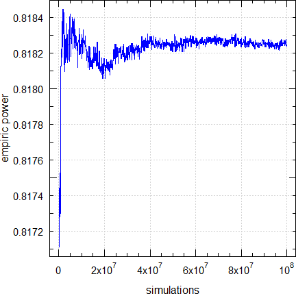
Fig. 2 Empiric power for n = 28.
In the Monte Carlo method values approach the exact one asymptotically.
Q: Why give links to some references an HTTP-error 404 ‘Not found’?
A: I checked all URLs in July 2024. Contrary to us mere mortals who have to maintain a document history, agencies don’t care. They change the structure of their websites (worst is the one of the WHO), don’t establish automatic redirects, delete or rename files… Quod licet Iovi, non licet bovi
Please drop me a note at [email protected].Q: I still have questions. How to proceed?
A: The preferred method is to register at the BEBA Forum and post your question in the category (please read the Forum’s Policy first).
You can contact me at [email protected]. Be warned – I will charge you for anything beyond most basic questions.
Abbreviations
| Abbreviation | Meaning |
|---|---|
| (A)BE | (Average) Bioequivalence |
| \(\small{CV_\textrm{inter}}\) | Between-subject Coefficient of Variation |
| \(\small{CV_\textrm{intra}}\) | Within-subject Coefficient of Variation (also ISCV) |
| \(\small{CV_\textrm{wT},\,CV_\textrm{wR}}\) | Within-subject Coefficient of Variation of the Test and Reference treatment |
| \(\small{H_0}\) | Null hypothesis |
| \(\small{H_1}\) | Alternative hypothesis (also \(\small{H_\textrm{a}}\)) |
| HVD(P) | Highly Variable Drug (Product) |
| NTID | Narrow Therapeutic Index Drug |
| RSABE | Reference-scaled Average Bioequivalence |
| TOST | Two One-Sided Tests |
| \(\small{\alpha}\) | Nominal level of the test, probability of Type I Error, patient’s risk |
| \(\small{\beta}\) | Probability of Type II Error, producer’s risk |
| \(\small{\pi}\) | Prospective power (\(\small{1-\beta}\)) |
Licenses
 Helmut Schütz 2024
R and PowerTOST GPL 3.0,
klippy MIT,
pandoc GPL 2.0.
1st version March 12, 2021. Rendered July 24, 2024 14:52 CEST
by rmarkdown
via pandoc in 0.86 seconds.
Footnotes and References
Labes D, Schütz H, Lang B. PowerTOST: Power and Sample Size for (Bio)Equivalence Studies. Package version 1.5.6. 2024-03-18. CRAN.↩︎
Labes D, Schütz H, Lang B. Package ‘PowerTOST’. March 18, 2024. CRAN.↩︎
Senn S. Guernsey McPearson’s Drug Development Dictionary. April 21, 2020. Online.↩︎
Hoenig JM, Heisey DM. The Abuse of Power: The Pervasive Fallacy of Power Calculations for Data Analysis. Am Stat. 2001; 55(1): 19–24. doi:10.1198/000313001300339897.
 Open
Access.↩︎
Open
Access.↩︎In short: There is no statistical method to ‘correct’ for unequal carryover. It can only be avoided by design, i.e., a sufficiently long washout between periods. According to the guidelines subjects with pre-dose concentrations > 5% of their Cmax can by excluded from the comparison if stated in the protocol.↩︎
Especially important for drugs which are auto-inducers or -inhibitors and biologics.↩︎
Senn S. Statistical Issues in Drug Development. Chichester: John Wiley; 2nd ed 2007.↩︎
Senn S. Statistical Issues in Drug Development. Chichester: John Wiley; 2004.↩︎
Zhang P. A Simple Formula for Sample Size Calculation in Equivalence Studies. J Biopharm Stat. 2003; 13(3): 529–38. doi:10.1081/BIP-120022772.↩︎
Doyle AC. The Adventures of Sherlock Holmes. A Scandal in Bohemia. 1892. p. 3.↩︎
Schütz H. Sample Size Estimation in Bioequivalence. Evaluation. 2020-10-23. BEBA Forum.↩︎
Lenth RV. Two Sample-Size Practices that I Don’t Recommend. October 24, 2000. Online.↩︎
Quoting my late father: »If you believe, go to church.«↩︎
Ring A, Lang B, Kazaroho C, Labes D, Schall R, Schütz H. Sample size determination in bioequivalence studies using statistical assurance. Br J Clin Pharmacol. 2019; 85(10): 2369–77. doi:10.1111/bcp.14055.
Open
Access.↩︎Berger RL, Hsu JC. Bioequivalence Trials, Intersection-Union Tests and Equivalence Confidence Sets. Stat Sci. 1996; 11(4): 283–302. JSTOR:2246021.↩︎
Zeng A. The TOST confidence intervals and the coverage probabilities with R simulation. March 14, 2014. Online.↩︎
With
alpha = 0.5the test effectively reduces to a dichotomous (pass|fail) assessment.↩︎The FDA and China’s CDE recommend Reference-Scaled Average Bioequivalence (RSABE) and a comparison of the within-subject variances of treatments. Details are covered in another article.↩︎
Owen DB. A special case of a bivariate non-central t-distribution. Biometrika. 1965; 52(3/4): 437–46. doi:10.2307/2333696.↩︎
The R Foundation for Statistical Computing. A Guidance Document for the Use of R in Regulated Clinical Trial Environments. Vienna. October 18, 2021. Online.↩︎
The R Foundation for Statistical Computing. R: Software Development Life Cycle. A Description of R’s Development, Testing, Release and Maintenance Processes. Vienna. October 18, 2021. Online.↩︎
Jiang W, Makhlouf F, Schuirmann DJ, Zhang X, Zheng N, Conner D, Yu LX, Lionberger R. A Bioequivalence Approach for Generic Narrow Therapeutic Index Drugs: Evaluation of the Reference-Scaled Approach and Variability Comparison Criterion. AAPS J. 2015; 17(4): 891–901. doi:10.1208/s12248-015-9753-5.
 Free
Full Text.↩︎
Free
Full Text.↩︎FDA. Statistical Software Clarifying Statement. May 6, 2015. Online.↩︎
WHO. Guidance for organizations performing in vivo bioequivalence studies. Geneva. May 2016. Technical Report Series No. 996, Annex 9. Section 4. Online.↩︎
ICH. Good Clinical Practice (GCP). E6(R3) – Draft. 19 May 2023. Section 4.5. Online.↩︎
Zheng C, Wang J, Zhao L. Testing bioequivalence for multiple formulations with power and sample size calculations. Pharm Stat. 2012; 11(4): 334–41. doi:10.1002/pst.1522.↩︎